Lecture: Describing Your Data

Mean, spread, counting correctly, and group summaries

Bill Perry

Where We Left Off

Last time you:

Imported data two ways (read_csv(), read_excel())
Wrangled with filter(), select(), mutate(), arrange()
Caught duplicate rows with distinct()
Saved a new file with write_csv()

Note

✅ Key idea from Wrangling Your Data

You can reshape a dataset and hand off a clean file. Today we start describing it — the step that comes before any formal test.

Note

Today’s roadmap

Mean and median
Variance and standard deviation
Quantiles, range, and IQR
The length() trap — and the fix
Standard error
skimr — a fast full-dataset overview
group_by() + summarize()

Part 1 · Our Question, Revisited

Our Question, Revisited

H₀: No difference in needle length between the shady and sunny sides
Hₐ: Needle length differs between the two sides

Before we can formally test that with statistics, we need to describe what we actually measured.

Note

Plan for this unit

Today — describe the data: center, spread, and group summaries
A later module — formally test H₀ vs. Hₐ

library(tidyverse)

pine_df <- read_csv("data/pine_needles.csv")

Tip

🖐 Recap

n_s codes shady (n) vs. sunny (s); group is the field team name.
Four teams, four trees, six needles per side.

Part 2 · The Mean

The Mean

\[\bar{x} = \frac{\sum_{i=1}^{n} x_i}{n}\]

Add up every value, divide by n
The balance point of the distribution
Sensitive to outliers — one very large value disproportionately affects the mean

Example: Values 5, 6, 7, 8, 50 → mean = 15.2.
Is that a fair summary?
Not really — the outlier dominates.

Note

✅ Why it matters

The mean is the most commonly reported statistic
— and it’s the number every t-test, ANOVA, and regression is ultimately built around.

# Pull one side's values out as a vector -----
shady_lengths <- pine_df |>
  filter(n_s == "n") |>
  pull(length_mm)

shady_lengths

 [1] 20 21 23 25 21 16 19 18 20 23 21 18 20 21 23 25 21 16 19 18 20 23 21 18

mean(shady_lengths)

[1] 20.41667

Tip

📖 New pattern

filter() picks rows. pull() extracts one column as a plain vector, not a data frame.

Part 3 · The Median

The Median

The middle value once the data are sorted

Sorted data	Median
5, 6, 7, 8, 50	7
5, 6, 7, 8, 50, 51	(7 + 8) / 2 = 7.5

Not pulled around by outliers — it’s robust
If mean ≫ median → right-skewed data
If mean ≈ median → roughly symmetric

sunny_lengths <- pine_df |>
  filter(n_s == "s") |>
  pull(length_mm)

median(shady_lengths)

[1] 20.5

median(sunny_lengths)

[1] 15

Note

✅ Key idea

Report mean and median together the first time you look at a new variable — a big gap between them is a signal worth investigating.

Part 4 · Variance (s²) and Standard Deviation (sd)

Variance and Standard Deviation

\[s^2 = \frac{\sum_{i=1}^{n}(x_i - \bar{x})^2}{n - 1} \qquad s = \sqrt{s^2}\]

Distance of each value from the mean
Square it — makes everything positive
Average those squared distances (over \(n-1\))
Square root brings variance back into the original units as the standard deviation

Larger spread = larger variance and SD.

Note

Variance is in squared units (mm²)
hard to interpret directly.
Standard deviation (SD) is why we usually report it instead

var(shady_lengths)

[1] 5.992754

sd(shady_lengths)

[1] 2.44801

var(sunny_lengths)

[1] 3.644928

sd(sunny_lengths)

[1] 1.909169

Tip

📖 Rule of thumb

For roughly normal data:
- ~68% of values fall within mean ± 1 SD
- ~95% within mean ± 2 SD

Part 4b · Quantiles, Range, and IQR

Quantiles, Range, and IQR

range(shady_lengths)              # min and max

[1] 16 25

max(shady_lengths) - min(shady_lengths)  # range as a single number

[1] 9

quantile(shady_lengths)           # 0/25/50/75/100th percentiles

   0%   25%   50%   75%  100% 
16.00 18.75 20.50 21.50 25.00

IQR(shady_lengths)                # 75th percentile minus 25th

[1] 2.75

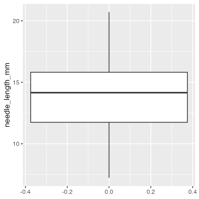
box_plot_1 <- ggplot(data = NULL, aes(y = shady_lengths)) + 
  geom_boxplot()

Note

✅ Key idea

The IQR is the range of the middle 50% of the data — it ignores the most extreme quarter on each end, which makes it robust to outliers the same way the median is.

Tip

🖐 Notice

quantile()’s 50th percentile is exactly the median. IQR() is just quantile(x, 0.75) - quantile(x, 0.25) computed for you.

📖 R4DS §12 — EDA

box_plot_1

Quantiles — Why This Matters for Graphing Effectively

quantile(sunny_lengths)

   0%   25%   50%   75%  100% 
12.00 13.75 15.00 16.00 19.00

IQR(sunny_lengths)

[1] 2.25

Tip

📖 Preview

The box in a boxplot is the IQR — its bottom and top edges are the 25th and 75th percentiles you just computed. The boxplots you’ll build in Graphing Effectively are these five numbers, drawn.

Part 5 · The `length()` Trap

The `length()` Trap

Important

🔮 Predict first: A vector has 5 slots, but 2 are NA. What does length() return? What should your sample size be for a mean or SE calculation?

x <- c(4, 3, NA, 7, NA)   # a vector with missing values

length(x)          # counts every slot — including NAs!

[1] 5

sum(is.na(x))       # how many are missing?

[1] 2

Note

📖 New words

is.na(x) — TRUE where a value is missing
!is.na(x) — the flip: TRUE where a value is real
sum(!is.na(x)) — counts the real values = the correct n

The `length()` Trap — Why It Matters

# Using length() as n silently gives the WRONG answer
wrong_n  <- length(x)
wrong_se <- sd(x, na.rm = TRUE) / sqrt(wrong_n)

wrong_n

[1] 5

round(wrong_se, 3)

[1] 0.931

# note base r rounding is really odd - use round_half_up from janitor

Warning

⚠️ Watch out!

R will not warn you. length() happily returns 5 when only 3 values are real — a silent, common error.

Fix — `sum(!is.na())`

is.na(x)          # TRUE where NA

[1] FALSE FALSE  TRUE FALSE  TRUE

!is.na(x)         # flipped: TRUE where real

[1]  TRUE  TRUE FALSE  TRUE FALSE

sum(!is.na(x))    # count the TRUEs

[1] 3

Tip

Best practice: use sum(!is.na(x)) for n every time you compute an SE — even when you’re sure there are no missing values. Field data rarely stays that clean.

How it works, step by step:

is.na(x) → TRUE for each missing value
!is.na(x) → flips it to TRUE for real values
sum(...) → adds up the TRUEs (TRUE = 1)

📖 R4DS §18 — Missing Values

Fix — Applied to Real Data

# Applied to our real data — even with no NAs, make it a habit
n_shady  <- sum(!is.na(shady_lengths))
n_sunny <- sum(!is.na(sunny_lengths))

n_shady

[1] 24

n_sunny

[1] 24

Tip

Even when you’re confident a column has zero missing values, run it through sum(!is.na()) anyway — it costs nothing and field data rarely stays clean for long.

Part 6 · Standard Error

Standard Error

\[SE = \frac{s}{\sqrt{n}}\]

Measures how precisely you know the mean — not the spread of raw data
Gets smaller as n grows: more data → a more precise estimate of the mean

	Describes
SD	spread of individual data points
SE	precision of the sample mean

We report SE whenever we’re making a claim about a group mean.

se_shady  <- sd(shady_lengths)  / sqrt(n_shady)
se_sunny <- sd(sunny_lengths) / sqrt(n_sunny)

round(se_shady, 2)

[1] 0.5

round(se_sunny, 2)

[1] 0.39

Warning

⚠️ Watch out!

sqrt(length(x)) and sqrt(sum(!is.na(x))) give the same answer only when there are zero missing values. Don’t assume — check.

All Stats, One Group, Base R

n_l    <- sum(!is.na(shady_lengths))
mean_l <- mean(shady_lengths, na.rm = TRUE)
med_l  <- median(shady_lengths, na.rm = TRUE)
sd_l   <- sd(shady_lengths, na.rm = TRUE)
se_l   <- sd_l / sqrt(n_l)

cat("--- Shady side ---\n",
    "n      =", n_l, "\n",
    "Mean   =", round(mean_l, 2), "\n",
    "Median =", round(med_l, 2), "\n",
    "SD     =", round(sd_l, 2), "\n",
    "SE     =", round(se_l, 2), "\n")

--- Shady side ---
 n      = 24 
 Mean   = 20.42 
 Median = 20.5 
 SD     = 2.45 
 SE     = 0.5

Every function takes na.rm = TRUE
cat() prints clean, labeled output

Note

✅ Key idea

Copy-pasting this block for every group is exactly the repetition group_by() + summarize() exists to remove.

Part 6b · `skimr` — a Fast Full-Dataset Overview

`skimr` — Every Column, One Command

install.packages("skimr")   # once per machine

library(skimr)

skim(pine_df)

Data summary
Name	pine_df
Number of rows	48
Number of columns	6
_______________________
Column type frequency:
character	4
numeric	2
________________________
Group variables	None

Variable type: character

skim_variable	complete_rate	min	max	n_unique
date	1	7	7	1
group	1	5	11	4
n_s	1	1	1	2
sun	1	5	5	2

Variable type: numeric

skim_variable	n_missing	complete_rate	mean	sd	p0	p25	p50	p75	p100	hist
tree_no	0	1	2.50	1.13	1	1.75	2.5	3.25	4	▇▇▁▇▇
length_mm	0	1	17.67	3.53	12	15.00	17.5	20.25	25	▆▇▅▆▃

Note

✅ Key idea

skim() gives you n, missing count, mean, SD, and a tiny inline histogram for every numeric column — and counts for every character column — in one call. It’s the fastest way to sanity-check a dataset the moment you load it.

`skimr` — Doesn’t Replace, Just Speeds Up

# Same idea, restricted to numeric columns
pine_df |>
  select(length_mm, tree_no) |>
  skim()

Data summary
Name	select(pine_df, length_mm…
Number of rows	48
Number of columns	2
_______________________
Column type frequency:
numeric	2
________________________
Group variables	None

Variable type: numeric

skim_variable	n_missing	complete_rate	mean	sd	p0	p25	p50	p75	p100	hist
length_mm	0	1	17.67	3.53	12	15.00	17.5	20.25	25	▆▇▅▆▃
tree_no	0	1	2.50	1.13	1	1.75	2.5	3.25	4	▇▇▁▇▇

Warning

⚠️ Watch out!

skim() is a first look, not a final answer.
you can pipe groups into it to show that length_mm should be split by n_s
- for real per-group comparisons, you still need group_by() + summarize(), next.

Part 7 · Tidy Group Stats — `group_by()` + `summarize()`

Tidy Group Stats — `group_by()` + `summarize()`

Note

🔮 Predict first: How many rows will the result have? (Hint: how many values does n_s take?)

side_stats_df <- pine_df |>
  group_by(n_s) |>
  summarize(
    n       = sum(!is.na(length_mm)),
    mean_mm = round(mean(length_mm, na.rm = TRUE), 2),
    med_mm  = round(median(length_mm, na.rm = TRUE), 2),
    sd_mm   = round(sd(length_mm, na.rm = TRUE), 2),
    se_mm   = round(sd_mm / sqrt(n), 2)
  )

side_stats_df

# A tibble: 2 × 6
  n_s       n mean_mm med_mm sd_mm se_mm
  <chr> <int>   <dbl>  <dbl> <dbl> <dbl>
1 n        24    20.4   20.5  2.45  0.5 
2 s        24    14.9   15    1.91  0.39

group_by(n_s) splits the data by side
summarize() collapses each group to one row of stats
Both groups, one clean table — no copy-paste
A column you just created (sd_mm) can feed the next one (se_mm)

📖 R4DS §3.5 — summarize()

Grouping by More Than One Variable

team_stats_df <- pine_df |>
  group_by(group, n_s) |>
  summarize(
    n       = sum(!is.na(length_mm)),
    mean_mm = round(mean(length_mm, na.rm = TRUE), 2),
    se_mm   = round(sd(length_mm, na.rm = TRUE) / sqrt(n), 2),
    .groups = "drop"
  )

team_stats_df

# A tibble: 8 × 5
  group       n_s       n mean_mm se_mm
  <chr>       <chr> <int>   <dbl> <dbl>
1 cephalopods n         6    21    1.24
2 cephalopods s         6    15    0.58
3 crayfish    n         6    21    1.24
4 crayfish    s         6    15    0.58
5 salmon      n         6    19.8  0.79
6 salmon      s         6    12.8  0.4 
7 snail       n         6    19.8  0.79
8 snail       s         6    16.8  0.6

group_by(group, n_s) splits by field team, then side — one row per combination
.groups = "drop" turns off the grouping once you’re done — good habit, avoids surprises later

Tip

🖐 Notice

Four teams × two sides = 8 rows. Does every team show the same shady-vs-sunny pattern, or do some disagree?

Part 7b · Bringing Back `case_when()` from Wrangling Your Data

Summarizing the Categories You Built Last Class

Note

🔮 Predict first: We’re grouping by the size_class bins ("short"/"medium"/"long") from Wrangling Your Data’s case_when(). How many rows will the summary have?

size_class_stats_df <- pine_df |>
  mutate(
    size_class = case_when(
      length_mm < 16 ~ "short",
      length_mm < 20 ~ "medium",
      TRUE           ~ "long"
    )
  ) |>
  group_by(size_class) |>
  summarize(
    n       = sum(!is.na(length_mm)),
    mean_mm = round(mean(length_mm, na.rm = TRUE), 2),
    se_mm   = round(sd(length_mm, na.rm = TRUE) / sqrt(n), 2)
  )

size_class_stats_df

# A tibble: 3 × 4
  size_class     n mean_mm se_mm
  <chr>      <int>   <dbl> <dbl>
1 long          16    21.8  0.42
2 medium        17    17.3  0.28
3 short         15    13.7  0.3

Note

✅ Key idea

mutate() and group_by() + summarize() chain together like any other verbs — you don’t need to save the case_when() column separately first. This is the wrangling → describing pipeline in one block.

Wrap-up

Today you:

Computed mean and median, and know why they can disagree
Computed variance and SD by hand, with real formulas
Computed quantiles, range, and IQR — and saw the IQR is literally the boxplot’s box
Found the length() trap and fixed it with sum(!is.na())
Computed SE and know how it differs from SD
Got a fast full-dataset overview with skimr::skim()
Used group_by() + summarize() to get every group’s stats in one table — including the case_when() categories from Wrangling Your Data

Tip

🖐 Before next class

Finish the worksheet: compute n, mean, SD, and SE for length_mm grouped by n_s, and again grouped by group. Save the summary table with write_csv().

Note

Up next — Graphing Effectively

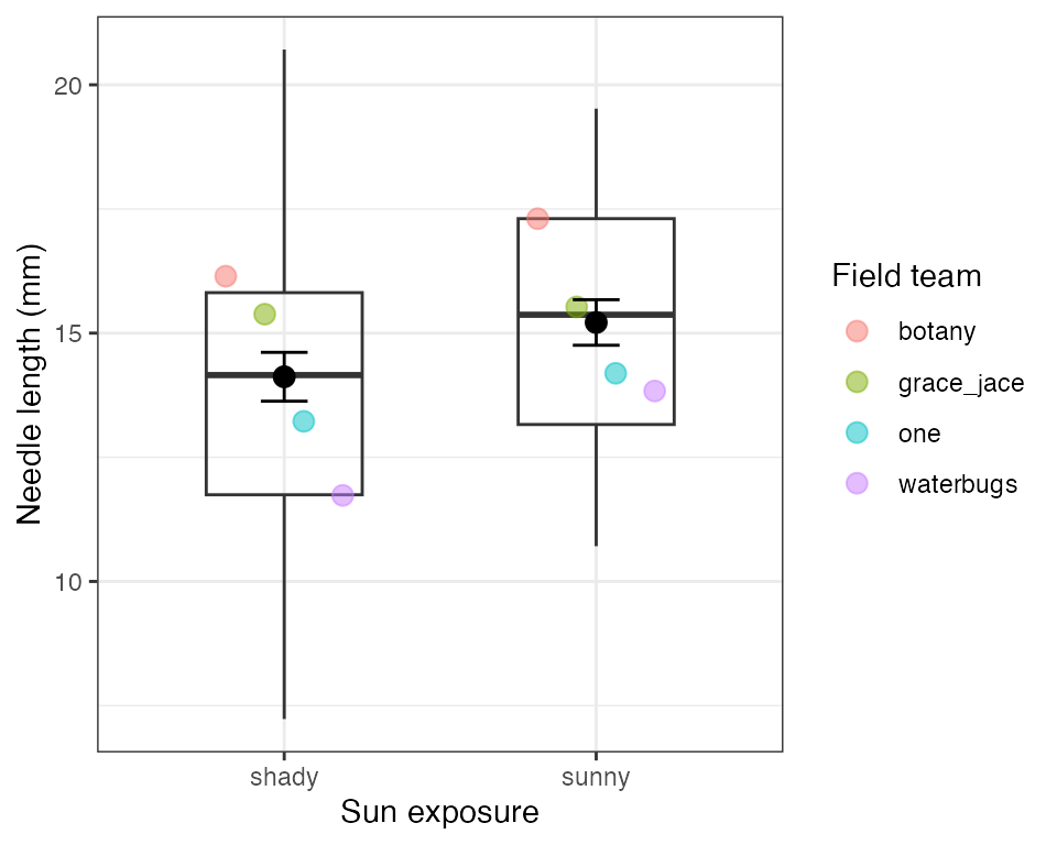
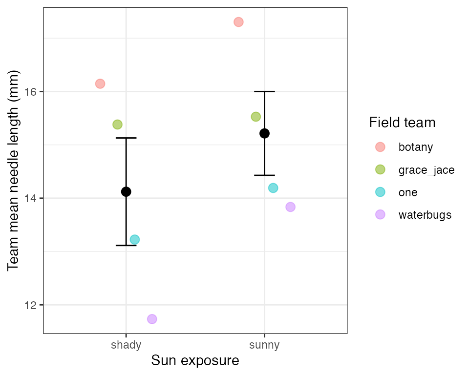
Boxplots and jittered points, done right
Plotting mean ± SE directly with stat_summary()
Faceting, themes, and ggsave() for a publication-ready figure

Getting unstuck

When code breaks — and it will, that is normal:

Read the error message out loud; it usually names the line
Check the usual suspects: library(tidyverse) loaded? Spelling? Did you forget na.rm = TRUE?
?function_name opens the help page
Bring the exact error (copy-paste it) to class or office hours

Note

✅ Key idea

Every working scientist googles error messages daily. Getting stuck is not failing — it is the job.

Lecture: Describing Your Data

Where We Left Off

Part 1 · Our Question, Revisited

Our Question, Revisited

Part 2 · The Mean

The Mean

Part 3 · The Median

The Median

Part 4 · Variance (s2) and Standard Deviation (sd)

Variance and Standard Deviation

Part 4b · Quantiles, Range, and IQR

Quantiles, Range, and IQR

Quantiles — Why This Matters for Graphing Effectively

Part 5 · The length() Trap

The length() Trap

The length() Trap — Why It Matters

Fix — sum(!is.na())

Fix — Applied to Real Data

Part 6 · Standard Error

Standard Error

All Stats, One Group, Base R

Part 6b · skimr — a Fast Full-Dataset Overview

skimr — Every Column, One Command

skimr — Doesn’t Replace, Just Speeds Up

Part 7 · Tidy Group Stats — group_by() + summarize()

Tidy Group Stats — group_by() + summarize()

Grouping by More Than One Variable

Part 7b · Bringing Back case_when() from Wrangling Your Data

Summarizing the Categories You Built Last Class

Wrap-up

Getting unstuck

Part 4 · Variance (s²) and Standard Deviation (sd)

Part 5 · The `length()` Trap

The `length()` Trap

The `length()` Trap — Why It Matters

Fix — `sum(!is.na())`

Part 6b · `skimr` — a Fast Full-Dataset Overview

`skimr` — Every Column, One Command

`skimr` — Doesn’t Replace, Just Speeds Up

Part 7 · Tidy Group Stats — `group_by()` + `summarize()`

Tidy Group Stats — `group_by()` + `summarize()`

Part 7b · Bringing Back `case_when()` from Wrangling Your Data