Lecture: Multiple Regression

Several predictors

Bill Perry

Where We Left Off

Covered last time:

• One continuous predictor, one continuous response
• The sums-of-squares partition: \(SS_{total} = SS_{regression} + SS_{residual}\)
• Mean squares, the F-ratio, and t² = F
• The four assumptions, all checked on the residuals

Note

✅ Key idea from last lecture

A simple regression has one predictor and one partition of variance. Today we add more predictors.

The logic barely changes. The bookkeeping does — and so does what each slope means.

Part 1 · Why Multiple Regression?

Today’s Objectives

The multiple linear regression model:

• Partial regression slopes — and why they are not the same as simple slopes
• Analysis of variance and the null hypotheses
• Assumptions, diagnostics and collinearity
• Interactions
• Factors, dummy variables, and choosing your reference level
• Model comparison and predictor importance

📥 Bird data 📥 Script skeleton (.R)

Note

📖 Reading

Quinn & Keough, Ch. 6 — Multiple and Complex Regression.

Whitlock & Schluter, Ch. 17; Gotelli & Ellison, Ch. 9.

The Study · Birds in Fragmented Forest

Loyn (1987) surveyed 56 remnant forest patches in Victoria, Australia, and counted the birds in each one. For every patch he also recorded six things that might explain the count.

Small patches, isolated patches, recently cut-off patches and heavily grazed patches are all candidates — and they are not independent of each other.

Column	What it is
abundance	birds per patch (the response)
area_ha	patch area
dist_m	distance to nearest patch
dist_larger_m	distance to nearest larger patch
year_isolated	year the patch was cut off
grazing	grazing intensity, 1–5
altitude_m	elevation

Reading the Data In

bird_df <- read_csv("data/loyn_birds.csv") %>%
  mutate(log_area        = log10(area_ha),
         log_dist        = log10(dist_m),
         log_dist_larger = log10(dist_larger_m))

glimpse(bird_df)

Rows: 56
Columns: 11
$ abundance       <dbl> 5.3, 2.0, 1.5, 17.1, 13.8, 14.1, 3.8, 2.2, 3.3, 3.0, 2…
$ area_ha         <dbl> 0.1, 0.5, 0.5, 1.0, 1.0, 1.0, 1.0, 1.0, 1.0, 1.0, 2.0,…
$ year_isolated   <dbl> 1968, 1920, 1900, 1966, 1918, 1965, 1955, 1920, 1965, …
$ dist_m          <dbl> 39, 234, 104, 66, 246, 234, 467, 284, 156, 311, 66, 93…
$ dist_larger_m   <dbl> 39, 234, 311, 66, 246, 285, 467, 1829, 156, 571, 332, …
$ grazing         <dbl> 2, 5, 5, 3, 5, 3, 5, 5, 4, 5, 3, 5, 2, 1, 5, 5, 3, 3, …
$ altitude_m      <dbl> 160, 60, 140, 160, 140, 130, 90, 60, 130, 130, 210, 16…
$ grazing_class   <chr> "light", "intense", "intense", "moderate", "intense", …
$ log_area        <dbl> -1.0000000, -0.3010300, -0.3010300, 0.0000000, 0.00000…
$ log_dist        <dbl> 1.591065, 2.369216, 2.017033, 1.819544, 2.390935, 2.36…
$ log_dist_larger <dbl> 1.591065, 2.369216, 2.492760, 1.819544, 2.390935, 2.45…

The three area and distance columns are logged on the way in.

That is not a stylistic choice — Part 4 shows what the raw scale does to the residuals, and it is the same failure you met in last week’s homework.

Note

grazing_class

The same grazing intensity as a word rather than a number. Part 7 is about what changes when you use it.

When Do We Need More Than One Predictor?

Bird abundance in a patch plausibly depends on all seven of those things at once, and they are not independent of each other — small patches tend to be grazed harder, and isolated patches tend to be older.

Fitting one predictor at a time cannot answer “does area matter once grazing is accounted for.”

• Predictors all continuous → multiple regression
• A mix of continuous and categorical → still multiple regression, with dummy variables

	Continuous X	Categorical X
Continuous Y	Regression	ANOVA
Categorical Y	Logistic regression	Contingency tables

One Predictor at a Time

Start the way you would have last week — fit each predictor on its own.

# A tibble: 6 × 3
  predictor         slope        p
  <chr>             <dbl>    <dbl>
1 log_area         9.78   7.18e-11
2 log_dist         3.29   3.52e- 1
3 log_dist_larger  2.21   3.86e- 1
4 year_isolated    0.211  7.68e- 5
5 grazing         -4.98   6.90e- 9
6 altitude_m       0.0952 3.32e- 3

Four of the six are significant on their own, two of them overwhelmingly.

Grazing looks like the strongest story in the dataset: every extra step of grazing intensity costs about 5 birds, at p = 6.90e-09.

Warning

⚠️ Hold that thought

Every one of these fits ignores the other five predictors entirely.

🗳️ DECIDE · Which Predictors Will Survive?

We are about to put all six predictors into one model together.

What do you expect to happen?

(a) All four significant predictors stay significant — they were each real

(b) Roughly the same four stay, but with smaller slopes

(c) Only one or two survive, and at least one strong predictor becomes non-significant

(d) Nothing survives — with six predictors and 56 patches there is not enough data

Warning

✍️ Write your letter down, then vote.

Note

The question to ask

How much of what grazing “explains” on its own is really being explained by patch area?

Small patches are grazed harder. Look back at the table — is grazing telling you something area was not already telling you?

From a Line to a (Hyper)plane

With one predictor we fit a line through a scatterplot.

With two, we fit a plane through a cloud — here, bird abundance over log patch area and grazing intensity.

With three or more it is a hyperplane, which you cannot draw but can still fit.

Part 2 · The Multiple Regression Model

The Multiple Regression Model

For i = 1 to n observations and p predictors:

\[y_i = \beta_0 + \beta_1 x_{i1} + \beta_2 x_{i2} + \dots + \beta_p x_{ip} + \epsilon_i\]

• \(y_i\) — the response for observation i
• \(\beta_0\) — the intercept, the mean of Y when every predictor is 0
• \(\beta_1 \dots \beta_p\) — the partial regression slopes
• \(\epsilon_i\) — the error, estimated by the residual \(y_i - \hat{y}_i\)

Note

✅ Key idea — what “partial” means

A partial slope is the change in Y per one-unit change in that predictor while every other predictor is held constant.

It is a conditional statement. Change what else is in the model and you have changed the condition — so the number is allowed to change too.

The Full Model · The Answer to the Vote

full_model <- lm(abundance ~ log_area + log_dist +
                   log_dist_larger + year_isolated +
                   grazing + altitude_m,
                 data = bird_df)

summary(full_model)

Call:
lm(formula = abundance ~ log_area + log_dist + log_dist_larger + 
    year_isolated + grazing + altitude_m, data = bird_df)

Residuals:
     Min       1Q   Median       3Q      Max 
-15.6506  -2.9390   0.5289   2.5353  15.2842 

Coefficients:
                  Estimate Std. Error t value Pr(>|t|)    
(Intercept)     -125.69725   91.69228  -1.371   0.1767    
log_area           7.47023    1.46489   5.099 5.49e-06 ***
log_dist          -0.90696    2.67572  -0.339   0.7361    
log_dist_larger   -0.64842    2.12270  -0.305   0.7613    
year_isolated      0.07387    0.04520   1.634   0.1086    
grazing           -1.66774    0.92993  -1.793   0.0791 .  
altitude_m         0.01951    0.02396   0.814   0.4195    
---
Signif. codes:  0 '***' 0.001 '**' 0.01 '*' 0.05 '.' 0.1 ' ' 1

Residual standard error: 6.384 on 49 degrees of freedom
Multiple R-squared:  0.6849,    Adjusted R-squared:  0.6464 
F-statistic: 17.75 on 6 and 49 DF,  p-value: 8.443e-11

Important

✅ The answer is (c).

Four predictors were significant alone. In the model together, only log_area survives (p < 0.001).

Grazing has gone from a slope of -4.98 (p = 6.90e-09) to -1.67 (p = 0.0791) — most of what grazing appeared to explain was patch area wearing a different hat.

Year of isolation and altitude have gone the same way.

Why Not Just Regress Y on Each X Separately?

Each simple regression asks “does this predictor track abundance?” The multiple regression asks “does it track abundance among patches that are otherwise alike?”

Those are different questions, and they can have different answers.

Predictor	Alone	In the full model
log area	9.78	7.47
grazing	-4.98	-1.67
year isolated	0.211	0.074
altitude	0.095	0.02

Warning

⚠️ Neither number is “wrong”

If you want to predict bird abundance from grazing alone, -4.98 is the right slope to use.

If you want to claim grazing has an effect beyond the fact that grazed patches are small, -1.67 is the number you have to defend — and here you cannot.

Estimation and Prediction

Estimation. Ordinary least squares again: choose the coefficients that minimise \(\sum(y_i - \hat{y}_i)^2\). With several predictors this is a set of simultaneous equations solved with matrix algebra — lm() does it instantly, and what matters is knowing what it minimises.

Prediction. Substitute new values for every predictor.

• More observations → narrower intervals
• More predictors → wider intervals
• Stay inside the range of every predictor

Warning

⚠️ Extrapolation is worse here

In simple regression you only have to stay inside one range. Here you have to stay inside the data cloud — and a combination can be far outside it even when each predictor separately looks ordinary.

There are no 1000-ha patches under intense grazing in these data. The model will still happily predict one.

Part 3 · ANOVA for Multiple Regression

Partitioning Variance — Sums of Squares

Exactly the partition from last week, with p predictors instead of one:

\[SS_{total} = SS_{regression} + SS_{residual}\]

• \(SS_{regression}\) — variation the model explains
• \(SS_{residual}\) — variation it does not
• Regression df is now p, not 1

Source	SS	df	MS
Regression	\(\sum (\hat{y}_i - \bar{y})^2\)	\(p\)	SS/df
Residual	\(\sum (y_i - \hat{y}_i)^2\)	\(n-p-1\)	SS/df
Total	\(\sum (y_i - \bar{y})^2\)	\(n-1\)

Mean squares are variances, so they do not grow with n — which is why the F-ratio is built from them and not from the sums of squares directly.

Hypotheses — the “Basic” Test

The overall F-test at the bottom of summary() tests one null:

\[H_0: \beta_1 = \beta_2 = \dots = \beta_p = 0\]

• If it is true, \(MS_{regression}\) and \(MS_{residual}\) estimate the same variance and F ≈ 1
• If any β is non-zero, \(MS_{regression}\) is inflated and F > 1

It tells you the model as a whole explains something. It does not tell you which predictor did the work.

Warning

⚠️ A significant overall F with nothing significant inside it

This happens, and it is the classic signature of collinearity: the predictors jointly explain a lot, but they are so tangled that no individual slope can be pinned down.

Hypotheses — Testing One Predictor

To ask whether one specific β is zero, fit the model with and without it and compare:

\[SS_{extra} = SS_{regression}^{full} - SS_{regression}^{reduced}\]

\[F_{1,\,n-p-1} = \frac{MS_{extra}}{MS_{residual}^{full}}\]

reduced_model <- lm(abundance ~ log_area + grazing,
                    data = bird_df)

anova(reduced_model, full_model)

Analysis of Variance Table

Model 1: abundance ~ log_area + grazing
Model 2: abundance ~ log_area + log_dist + log_dist_larger + year_isolated + 
    grazing + altitude_m
  Res.Df    RSS Df Sum of Sq     F Pr(>F)
1     53 2200.9                          
2     49 1996.8  4    204.09 1.252 0.3015

Dropping four predictors at once — distance, distance to a larger patch, year of isolation and altitude — costs nothing detectable (p = 0.302).

Tip

🖐 You rarely run this by hand

The t-test beside each coefficient in summary() answers the same question for a single predictor. Use anova() when you want to drop a group of predictors at once.

Explained Variance

\[R^2 = \frac{SS_{regression}}{SS_{total}} = 1 - \frac{SS_{residual}}{SS_{total}}\]

For the reduced model: \(\dfrac{4137}{6338}\) = 0.653

The six-predictor model manages 0.685 — higher, as it must be.

Warning

⚠️ Watch out

• R² always rises when you add a predictor, even a useless one
• So R² cannot be used to compare models with different numbers of predictors
• R² from models with differently transformed Y are not comparable at all

That is why adjusted R² and AIC exist, and we come back to them in Part 8.

Part 4 · Assumptions and Diagnostics

First: Does a Predictor Need a Transform?

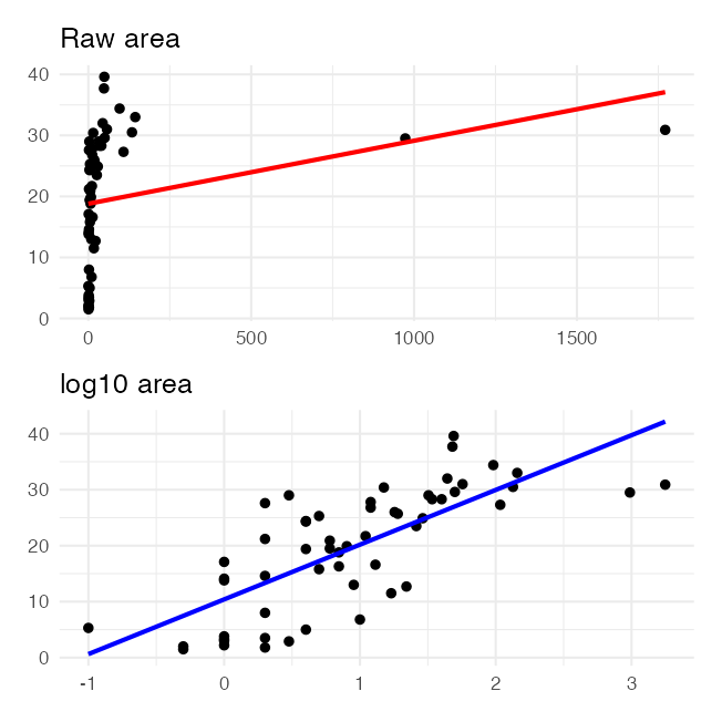
Patch area runs from 0.1 ha to 1,771 ha — four orders of magnitude. Fitted raw, it behaves exactly like last week’s homework:

	raw area_ha	log10(area_ha)
slope	0.0103	9.78
R²	0.066	0.548
Shapiro on residuals	0.014	0.0831

Every model in this lecture uses log_area, and the diagnostics are why.

Assumptions and Diagnostics — Outliers

• Fixed X values — unrealistic in field data, but the working assumption
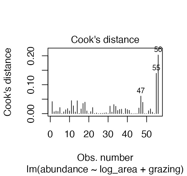
• No overly influential points — check leverage and influence with Cook’s distance
• A point can be extreme in Y, extreme in X, or extreme in the combination; only the third kind is uniquely a multiple-regression problem

Largest Cook’s distance here is 0.2 — nothing near the usual threshold of 1.

plot(reduced_model, which = 4)

Assumptions and Diagnostics — Residuals

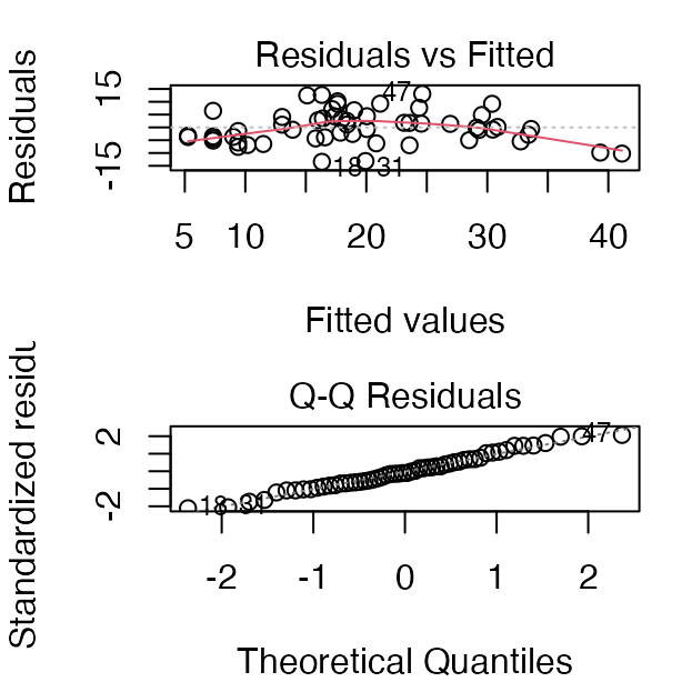
Normality, equal variance and independence — all read off the residuals, exactly as last week.

shapiro.test(residuals(reduced_model))

    Shapiro-Wilk normality test

data:  residuals(reduced_model)
W = 0.98422, p-value = 0.6728

Distribution and variance problems are usually fixed by transforming Y, or a predictor, before anything more exotic.

Assumptions — Sample Size and Added-Variable Plots

• More observations than predictors — a common rule of thumb is 10 observations per predictor. Six predictors would want 60; we have 56, so the full model is already at the edge
• Predictors not collinear — Part 5
• Each X linear in Y after accounting for the others — this is what an added-variable plot shows, and it is the multiple-regression version of “plot your data first”

avPlots(reduced_model)

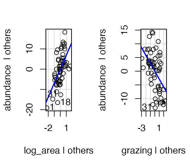
Each panel is Y and one X after the other predictor’s effect has been removed from both.

Part 5 · Collinearity

Collinearity — the Problem

Predictors in field data are almost never independent. Here, small patches are grazed harder — r = -0.56.

When predictors overlap:

• Parameter estimates become unstable — one changed value can move them a lot
• Standard errors inflate, so slopes lose significance
• The model can fit well while no single slope is trustworthy

                log_area log_dist log_dist_larger year_isolated grazing
log_area            1.00     0.30            0.38          0.28   -0.56
log_dist            0.30     1.00            0.60         -0.02   -0.14
log_dist_larger     0.38     0.60            1.00         -0.16   -0.03
year_isolated       0.28    -0.02           -0.16          1.00   -0.64
grazing            -0.56    -0.14           -0.03         -0.64    1.00
altitude_m          0.28    -0.22           -0.27          0.23   -0.41
                altitude_m
log_area              0.28
log_dist             -0.22
log_dist_larger      -0.27
year_isolated         0.23
grazing              -0.41
altitude_m            1.00

Collinearity — Detecting It

Variance Inflation Factors:

\[VIF_{X_j} = \frac{1}{1 - R^2_j}\]

where \(R^2_j\) comes from regressing \(X_j\) on all the other predictors — not from a pairwise correlation. (With two predictors they coincide; with more they do not.)

• Rule of thumb: VIF > 10 is bad; some authors use > 5
• Simplest fix: drop predictors that are measuring the same thing

vif(full_model)

       log_area        log_dist log_dist_larger   year_isolated         grazing 
       1.911514        1.654553        2.009749        1.804769        2.524814 
     altitude_m 
       1.467937 

Note

✅ Key idea

A high VIF does not mean the model is wrong. It means you cannot trust the individual partial slopes, even when the model as a whole fits well.

🗳️ DECIDE · The Slope That Changed Its Mind

Grazing went from -4.98 on its own to -1.67 in the full model, and lost its significance. The VIFs are all under 3.

What is the right thing to say about grazing?

(a) Grazing has no effect on bird abundance

(b) The effect of grazing is real but small — the full model estimates it better

(c) Grazing and patch area explain overlapping variation, and these data cannot cleanly separate them

(d) The full model is broken by collinearity and should be discarded

Warning

✍️ One letter. Write it down, then argue it with your neighbour.

Note

The question to ask

Is this a statement about the world, or a statement about what this dataset can resolve?

What the Data Can and Cannot Separate

Important

✅ The answer is (c).

Grazing and area are correlated at r = -0.56. The heavily grazed patches in this dataset are also the small ones, so no analysis can tell you which of the two is doing the work.

(a) overstates it — a non-significant partial slope is not evidence of no effect. (b) is the common mistake: the full model is not “better”, it answers a different, conditional question. (d) is wrong too — VIFs under 3 are mild, and the model predicts perfectly well. It just cannot apportion credit.

Tip

🖐 What would settle it

Find, or create, patches that break the correlation: large heavily grazed patches and small lightly grazed ones.

That is a design problem, not an analysis problem — which is where this course started.

Part 6 · Interactions

Interactions — Additive vs. Multiplicative

So far every model has been additive — the effect of area is the same at every grazing level.

An interaction says the effect of one predictor depends on the level of another:

\[y_i = \beta_0 + \beta_1X_{1} + \beta_2X_{2} + \epsilon_i\] \[y_i = \beta_0 + \beta_1X_{1} + \beta_2X_{2} + \beta_3X_{1}X_{2} + \epsilon_i\]

An interaction term is just another predictor: the product of two others, with its own coefficient.

Note

✅ Key idea

Additive: parallel lines.

Interactive: lines with different slopes — the fitted surface is no longer flat.

Interactions — Fitting One

interaction_model <- lm(abundance ~ log_area * grazing,
                        data = bird_df)

summary(interaction_model)$coefficients

                  Estimate Std. Error   t value     Pr(>|t|)
(Intercept)      26.558079  3.3576293  7.909771 1.768256e-10
log_area          2.112005  2.0375755  1.036528 3.047520e-01
grazing          -4.547139  0.8850592 -5.137667 4.246998e-06
log_area:grazing  2.142303  0.7358161  2.911465 5.287173e-03

The interaction is significant (p = 0.00529), and a * b expands to a + b + a:b automatically.

What it means: patch area matters more where grazing is heavy. In lightly grazed country a small patch still holds birds; under heavy grazing only the big patches do.

Warning

⚠️ You cannot read the main effects the same way any more

With an interaction in the model, the log_area coefficient is the slope when grazing = 0 — a value that does not exist in these data.

Interactions — the Cost

• Parameter proliferation. Every predictor you add roughly doubles the number of possible terms — six predictors with all interactions is 64 terms, and you have 56 patches
• Interpretation gets harder, as the slide before shows
• Include an interaction when it makes biological sense, not because it might be significant

“Does fragmentation hurt more where grazing is heavy” is a real hypothesis. That is why this one belongs.

Warning

⚠️ Watch out

Test enough interactions and one will reach p < 0.05 by chance. With six predictors there are 15 two-way interactions alone — at α = 0.05 you expect roughly one false positive just from testing them all.

Part 7 · Factors and Dummy Variables

Categorical Predictors Become Dummy Variables

So far grazing has been a number, 1 to 5, which forces every step to have the same effect. That is a strong assumption — is the jump from light to moderate really the same size as moderate to heavy?

Treat it as a category instead and the model estimates each level separately. A categorical predictor with k levels becomes k − 1 dummy variables, each 0 or 1.

One level gets no dummy at all. That is the reference level, and every other coefficient is a comparison against it.

count(bird_df, grazing, grazing_class)

# A tibble: 5 × 3
  grazing grazing_class     n
    <dbl> <chr>         <int>
1       1 minimal          13
2       2 light             8
3       3 moderate         15
4       4 heavy             7
5       5 intense          13

R Picks the Reference Level for You — Alphabetically

bird_df <- bird_df %>%
  mutate(grazing_class = factor(grazing_class))

levels(bird_df$grazing_class)

[1] "heavy"    "intense"  "light"    "minimal"  "moderate"

A character column becomes a factor in alphabetical order, so the reference level here is heavy — the fourth of five grazing intensities, chosen by spelling.

                      Estimate Std. Error t value Pr(>|t|)
(Intercept)              14.12       2.49    5.68     0.00
log_area                  7.25       1.26    5.77     0.00
grazing_classintense    -10.30       2.84   -3.62     0.00
grazing_classlight        1.97       3.05    0.65     0.52
grazing_classminimal      1.59       2.98    0.53     0.60
grazing_classmoderate     1.40       2.70    0.52     0.61

Every grazing coefficient is now “compared with heavy grazing,” which is a comparison nobody asked for.

🗳️ DECIDE · Which Level Should Be the Reference?

The five grazing classes are minimal, light, moderate, heavy, intense.

Which should be the reference level, and why?

(a) heavy — leave R’s default alone; the choice does not affect the model

(b) intense — the most extreme level makes the biggest contrasts

(c) minimal — the least-disturbed level, so every coefficient reads as the cost of adding grazing

(d) It does not matter, because R² and the F-test are identical either way

Warning

✍️ Careful — two of these are true statements. Only one is the right decision.

Note

The question to ask

Which comparison do I want to read straight off the output?

Choosing the Reference Yourself · fct_relevel()

Important

✅ The answer is (c).

4. is true — the fit, R², F and the ANOVA table are all identical whichever level is the reference. But it is not a reason to accept a bad default: the coefficients are what people read, and they should answer the question you asked.

minimal grazing is the closest thing this observational study has to a control, so putting it first makes every other coefficient “birds lost relative to the least-grazed patches.”

bird_df <- bird_df %>%
  mutate(grazing_class = fct_relevel(
    grazing_class,
    "minimal", "light", "moderate", "heavy", "intense"))

levels(bird_df$grazing_class)

[1] "minimal"  "light"    "moderate" "heavy"    "intense" 

Tip

🖐 The habit to build

Any time a factor enters a model, set its reference level on purpose, in the same line where you create the factor.

fct_relevel() moves the levels you name to the front and leaves the rest in place, so naming just the control is enough:

fct_relevel(treatment, "control")

Same Model, Same F, a Readable Story

grazing_model <- lm(abundance ~ log_area + grazing_class,
                    data = bird_df)

summary(grazing_model)$coefficients %>% round(2)

                      Estimate Std. Error t value Pr(>|t|)
(Intercept)              15.72       2.77    5.68     0.00
log_area                  7.25       1.26    5.77     0.00
grazing_classlight        0.38       2.91    0.13     0.90
grazing_classmoderate    -0.19       2.55   -0.07     0.94
grazing_classheavy       -1.59       2.98   -0.53     0.60
grazing_classintense    -11.89       2.93   -4.06     0.00

Now every coefficient is a comparison with minimal grazing, and the pattern is obvious:

• light, moderate and heavy are all indistinguishable from minimal
• intense costs about 11.9 birds, p < 0.001

Grazing is a threshold, not a gradient — and fitting it as the number 1–5 hid that completely, averaging the effect into -2.85 birds per step.

Why This Matters Even More in ANOVA

With only continuous predictors there is no reference level at all — every slope is “per unit of X” and nothing is being compared with anything.

The moment a factor enters the model, every coefficient becomes a contrast against the reference, and that is the whole structure of the next five weeks:

• One-way ANOVA — treatment means against a control
• Two-way ANOVA — main effects read at the other factor’s reference level
• ANCOVA — separate intercepts, all relative to one group

Important

✅ The rule to carry forward

factor() gives you alphabetical order. Alphabetical order is almost never the order your experiment was designed in.

Set the control as the first level, every time, and your model output reads as “what each treatment did to the control” without any further work.

Part 8 · Comparing Models

Comparing Models — the Problem

• Which predictors should be in the model?
• Occam’s razor: the best model balances fit against complexity
• Overfitting: a high R² bought with useless predictors — which is why R² alone cannot choose between models

Compare nested models: one whose predictors are a subset of the other’s.

Note

📖 Reference

Quinn & Keough, Ch. 6, works through exactly this dataset. Whitlock & Schluter, Ch. 17, covers model comparison for regression.

Comparing Models — Penalizing Complexity

Two ways to charge a model for its predictors:

\[\text{Adjusted } R^2 = 1 - \frac{SS_{Residual}/(n - p - 1)}{SS_{Total}/(n - 1)}\]

\[\text{AIC} = n\ln(SS_{Residual}) + 2(p + 1) - n\ln(n)\]

• Higher adjusted R² is better
• Lower AIC is better
• AIC is comparative only — the number on its own means nothing, and models must be fitted to the same rows

Warning

⚠️ The NA trap

If one predictor has missing values, lm() silently drops those rows. Two models fitted to different numbers of rows cannot be compared by AIC, and R will not warn you.

Comparing Models — How to Search

• Fit all possible models and compare — fine with a few predictors, hopeless with many
• Automated stepwise selection adds or removes terms by partial F or AIC
• We use manual backward selection: start full, drop what earns nothing, stop when dropping hurts

Warning

⚠️ Stepwise selection is controversial

It inflates R², biases p-values, and knows nothing about biology. A small set of models you can justify beats an automated search over all of them.

Comparing Models — Putting It Together

model_comparison <- tibble(
  model = c("all six predictors",
            "log_area + grazing",
            "log_area only",
            "grazing only"),
  adj_r2 = c(summary(full_model)$adj.r.squared,
             summary(reduced_model)$adj.r.squared,
             summary(lm(abundance ~ log_area, bird_df))$adj.r.squared,
             summary(lm(abundance ~ grazing, bird_df))$adj.r.squared),
  AIC = c(AIC(full_model),
          AIC(reduced_model),
          AIC(lm(abundance ~ log_area, bird_df)),
          AIC(lm(abundance ~ grazing, bird_df)))
) %>%
  mutate(delta_AIC = AIC - min(AIC)) %>%
  arrange(AIC)

model_comparison

# A tibble: 4 × 4
  model              adj_r2   AIC delta_AIC
  <chr>               <dbl> <dbl>     <dbl>
1 log_area + grazing  0.640  373.      0   
2 all six predictors  0.646  375.      2.55
3 log_area only       0.539  385.     12.8 
4 grazing only        0.456  395.     22.1 

Important

✅ The two-predictor model wins

It has the lowest AIC and essentially the same adjusted R² as the full model — with four fewer predictors.

A ΔAIC above about 2 is usually treated as a real difference, so the full model’s extra terms are not paying for themselves.

The anova() test in Part 3 said the same thing. Two routes, one answer.

Part 9 · Relative Importance of Predictors

How Important Is Each Predictor?

Three standard approaches, and they answer slightly different questions:

1. F- or t-tests on the partial slopes
2. Coefficient of partial determination — the variance a predictor adds
3. Standardized partial slopes — every predictor in SD units

None of them is “the” right answer.

Warning

⚠️ Why the raw slopes cannot be compared

log_area has a slope of 6.89 and grazing -2.85.

One is “birds per tenfold increase in area,” the other is “birds per step of grazing intensity.” Comparing those two numbers is comparing metres with kilograms.

Approaches 1 and 2 — Partial F and Partial R²

Anova(reduced_model, type = "II")

Anova Table (Type II tests)

Response: abundance
          Sum Sq Df F value    Pr(>F)    
log_area  1184.6  1  28.527 1.977e-06 ***
grazing    666.0  1  16.038 0.0001946 ***
Residuals 2200.9 53                      
---
Signif. codes:  0 '***' 0.001 '**' 0.01 '*' 0.05 '.' 0.1 ' ' 1

Partial η² = \(\dfrac{SS_{predictor}}{SS_{predictor} + SS_{residual}}\) — variance explained after controlling for the other predictor.

	log_area	grazing
partial η²	0.35	0.232
ΔR²	0.187	0.105

ΔR² is what the model’s R² would lose if you dropped that predictor — its unique contribution.

Both say area is the stronger of the two.

Approach 3 — Standardized Partial Slopes

Rescale every variable to mean 0 and SD 1, and the slopes become directly comparable: “SDs of Y per SD of X.”

bird_z <- bird_df %>%
  mutate(across(c(abundance, log_area, grazing),
                ~ as.numeric(scale(.))))

lm(abundance ~ log_area + grazing, data = bird_z) %>%
  coef() %>% round(3)

(Intercept)    log_area     grazing 
      0.000       0.521      -0.391 

log_area 0.52 versus grazing -0.39 — area is about 1.3× the influence of grazing per standard deviation.

Note

✅ All three agree here

Partial F, partial R² and standardized slopes all rank area above grazing. When they disagree, that is worth reporting — it usually means the predictors are tangled.

Wrap-up

Today you:

• Extended the regression line to a plane, and fitted 56 forest patches against six predictors at once
• Watched four predictors that were significant alone collapse to one in the model together
• Read a partial slope as a conditional statement, and saw that neither it nor the simple slope is “wrong”
• Tested groups of predictors with anova(reduced, full) and single ones with the t-tests in summary()
• Diagnosed collinearity with vif(), and learned to say “these data cannot separate them” instead of “it has no effect”
• Fitted a real interaction — fragmentation costs more where grazing is heavy
• Turned a categorical predictor into dummy variables, and set the reference level on purpose with fct_relevel()
• Compared models with adjusted R² and AIC, and ranked predictors three different ways

The Three Things to Carry Out of Here

Important

⚠️ R² always rises

Adding predictors can only increase plain R². Adjusted R² and AIC exist precisely because “explains more variance” is not the same as “is a better model.”

Note

✅ A partial slope is conditional

“What does area do among patches grazed the same amount?” Change what else is in the model and you have changed the question.

Important

✅ Set your reference level

factor() sorts alphabetically. Your control is almost never first alphabetically — use fct_relevel() and make the output say what you meant.

This is the habit that makes every ANOVA from Week 8 onward readable.

Note

Up next — Analysis of Variance

What happens when every predictor is categorical, and why ANOVA and regression are the same machinery in different clothes.

Readings

• Quinn, G. P., & Keough, M. J. (2002). Experimental Design and Data Analysis for Biologists, Ch. 6 — Multiple and Complex Regression. This lecture follows their Box 6-2 analysis of the Loyn data.
• Whitlock & Schluter, Ch. 17 — Regression.
• Gotelli & Ellison, Ch. 9 — Regression.
• Loyn, R. H. (1987). Effects of patch area and habitat on bird abundances, species numbers and tree health in fragmented Victorian forests. In Nature Conservation: The Role of Remnants of Native Vegetation. Surrey Beatty & Sons.

Getting unstuck

When code breaks — and it will, that is normal:

1. Read the error message out loud; it usually names the line
2. Check the usual suspects: is it y ~ x1 + x2 (additive) or y ~ x1 * x2 (interaction)? Is car loaded for vif() and Anova()? Are you comparing models fitted to the same rows — an NA in one predictor silently drops that row
3. ?function_name opens the help page
4. Bring the exact error (copy-paste it) to class or office hours

Note

✅ Key idea

Every working scientist googles error messages daily. Getting stuck is not failing — it is the job.