Lecture: NMDS & Cluster Analysis

Community ordination

Bill Perry

Part 1 · Why NMDS?

Introduction: Why NMDS?

The Problem with Ecological Community Data

  • Ecological community data presents unique challenges for traditional statistical methods
  • When sampling species abundances across sites
  • encounter data that is sparse (most species are absent from most sites) - many zeros
  • exhibits non-linear relationships between species and environmental gradients
  • has no clear distributional form
  • Principal Components Analysis (PCA) works beautifully for continuous environmental variables
    • assumes linear relationships
    • can leverage correlations between variables
    • for species abundance data - assumptions often fail spectacularly
  • NMDS offers a fundamentally different approach:
    • instead of trying to preserve exact distances or maximize variance explained

    • focuses on preserving the rank order of similarities between samples

    • makes it remarkably robust for ecological data.

NMDS - Multivariate Community Analysis

Data - built in R and other places

Code Description of the variable
das Distance from the source [km]
alt Altitude [m a.s.l.]
pen Slope [per thousand]
deb Mean minimum discharge [m3s-1]
pH pH of water
dur Calcium concentration (hardness) [mgL-1]
pho Phosphate concentration [mgL-1]
nit Nitrate concentration [mgL-1]
amn Ammonium concentration [mgL-1]
oxy Dissolved oxygen [mgL-1]
dbo Biological oxygen demand [mgL-1]
Code Common Name (English) Family
Chb Bullhead Cottidae
Tru Brown trout Salmonidae
Vai Minnow Cyprinidae
Loc Stone loach Balitoridae
Omb Grayling Salmonidae
Bla Souffia Cyprinidae
Hot Common nase Cyprinidae
Tox Sofie Cyprinidae
Van Dace Cyprinidae
Che Chub Cyprinidae
Bar Barbel Cyprinidae
Lot Burbot Lotidae
Spi Spirlin Cyprinidae
Gou Gudgeon Cyprinidae
Bro Pike Esocidae
Per Perch Percidae
Tan Tench Cyprinidae
Gar Roach Cyprinidae
Lam Brook lamprey petromizonidae

Today’s Data: The Doubs River

About the Doubs River Dataset

  • Study System:
    • Doubs River, France
    • 29 sites from upstream to downstream
    • Collected by Verneaux (1973)
    • Classic community ecology dataset
  • Two Datasets:
    1. Environmental: 11 water quality variables
    2. Species: 27 fish species abundances (0-5 scale)
  • Research Questions:
    • How do fish communities change along the river?
    • Which environmental factors drive community composition?
    • Are there distinct community types?

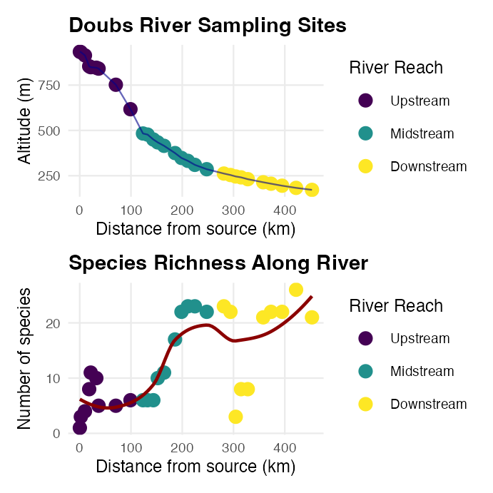
Two stacked plots of the Doubs River sampling design: altitude versus distance from source with points colored by river reach, and species richness versus distance from source with a loess smooth, both showing values changing as the river flows downstream.

Part 2 · The NMDS Algorithm

Non-metric Multidimensional Scaling (NMDS)

  • What is NMDS?
    • Overview of NMDS:
      • Purpose: Visualize dissimilarity between objects in 2D/3D space
      • Goal: Preserve rank order of distances, not exact distances
      • Method: Iterative re-positioning to minimize stress
      • Output: Ordination plot showing relationships between samples
    • Key Differences from PCA:
      • Uses dissimilarity matrices (not covariance)

      • Non-parametric (rank-based)

      • Better for non-linear ecological relationships

      • No assumption about data distribution

  • Before running NMDS - analyzing dissimilarity matrices not raw abundance data
    • dissimilarity matrix contains values for every pair of samples = “how different”

    • typically range from 0 (identical) to 1 (completely different).

Note

Gotelli & Ellison, A Primer of Ecological Statistics, Ch. 12 — The Analysis of Multivariate Data, covers ordination methods including NMDS.
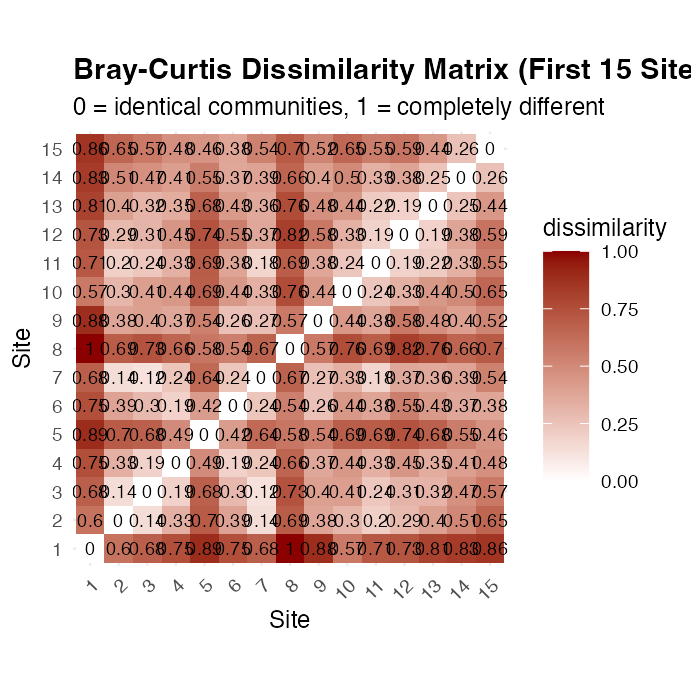
Heatmap of the Bray-Curtis dissimilarity matrix for the first 15 river sites, with cells colored from white (identical) to dark red (completely different) and dissimilarity values printed in each cell.

Why Bray-Curtis for Community Data?

  • Bray-Curtis dissimilarity is standard choice for community data because it handles zeros appropriately (joint absences don’t contribute to similarity)
    • bounded between 0 and 1

    • weights by abundance (not just presence/absence) - ignores joint absences entirely

    • Similarity is based only on what’s actually present and shared between sites

    • performs well with sparse data

The formula is:

\[BC_{jk} = \frac{\sum_i |y_{ij} - y_{ik}|}{\sum_i (y_{ij} + y_{ik})}\]

Where \(y_{ij}\) is the abundance of species \(i\) at site \(j\)

  • numerator sums up the absolute differences in abundance for each species between two sites
  • denominator sums up the total abundance at both sites
  • Bray-Curtis asks: “Of all the individuals at these two sites, what proportion would need to be moved to make the sites identical?”

The NMDS Algorithm

  • What NMDS Actually Does
    • NMDS tries to place samples in a low-dimensional space (usually 2D)
    • so rank order of distances in ordination matches rank order of dissimilarities in original matrix
  • Not your PCA which preserves exact distances (or variance)
  • NMDS only cares about relative ordering:
    • if site A is more similar to site B than to site C in the original data
    • then A should be closer to B than to C in the ordination

How NMDS Works step by step

  • The NMDS Algorithm:
    1. Calculate dissimilarity matrix between all pairs of sites
    2. Start with random configuration of points in 2D space
    3. Calculate stress = difference between original distances and ordination distances
    4. Move points to reduce stress
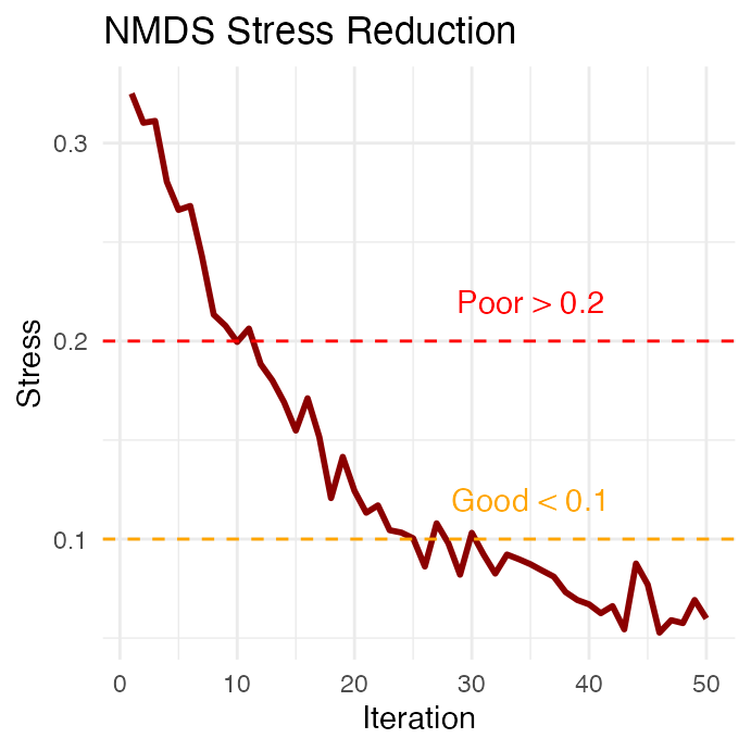
    5. Repeat until stress cannot be reduced further
    6. Try multiple random starts to avoid local minima
  • Stress Values:
    • < 0.1: Good representation
    • 0.1-0.2: Acceptable
    • > 0.2: Poor representation

Line plot of simulated NMDS stress declining over 50 iterations, with dashed reference lines at 0.1 (good threshold) and 0.2 (poor threshold).

Part 3 · Stress and Model Diagnostics

Understanding Stress

  • What is Stress?
    • Stress is key diagnostic for NMDS quality
    • measures disagreement between original dissimilarities and distances in ordination
    • stress is calculated by first ranking all pairwise dissimilarities
    • then calculating corresponding distances in the ordination
    • fitting a monotonic regression line to the relationship between these
    • finally computing sum of squared deviations from this line.
  • Lower stress means ordination better represents original relationships
  • The Shepard Diagram: Visualizing Stress
    • Shepard diagram (or stress plot) is primary diagnostic tool for NMDS
    • shows relationship between original dissimilarities (x-axis) and ordination distances (y-axis) with a fitted monotonic line
    • If NMDS is working well - points should closely follow the line
    • Scatter indicates loss of information.
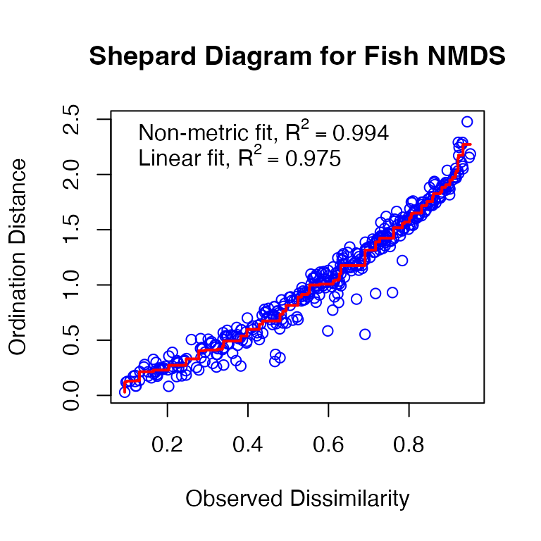
Shepard diagram for the fish NMDS: a scatterplot of ordination distance versus original Bray-Curtis dissimilarity for every pair of sites, with a stepped monotonic regression line, showing points closely tracking the line.

Interpreting the Shepard Diagram

  • Shepard diagram
    • each point represents one pair of sites
    • x-axis shows their original Bray-Curtis dissimilarity
    • y-axis shows their distance in the 2D ordination
    • stepped line is a monotonic regression, = can only go up/stay flat not down
    • because NMDS preserves rank order - “stress” = scatter around line
  • Insights from our Shepard diagram:
    • minimal scatter
  • Stress Guidelines
    • Clarke (1993) widely-used guidelines for interpreting stress
      • <0.05 excellent representation w/no misinterpretation
      • 0.05 - 0.10 good ordination - no real risk of false inferences
      • 0.10 - 0.20 usable ordination but details at lower end interpreted cautiously
      • 0.20 and 0.30 used with caution/potentially higher dimensions considered
      • >0.30 = random placement.

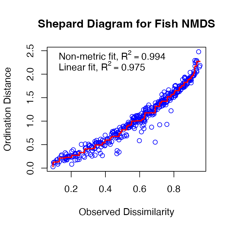
The same Shepard diagram for the fish NMDS repeated, shown alongside the discussion of stress guidelines for interpreting scatter around the monotonic line.

Choosing the Number of Dimensions

  • How do we know 2 dimensions is enough?
  • create a scree plot showing stress for different numbers of dimensions:
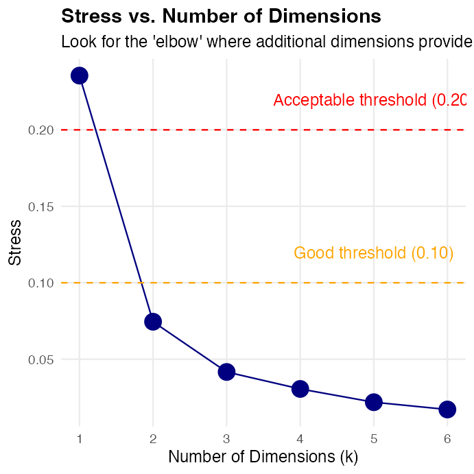
Scree plot of NMDS stress versus number of dimensions (1 to 6), with dashed reference lines at the 0.10 good and 0.20 acceptable stress thresholds, used to find the elbow where added dimensions stop meaningfully reducing stress.

NMDS Assumptions

  • NMDS Assumptions:
  • Few assumptions:
    • Samples are independent
    • Dissimilarity measure is appropriate
    • Sufficient data for stable solution
  • No assumptions about:
    • Data distribution
    • Linear relationships
    • Homoscedasticity
    • Normality
  • This makes NMDS very robust for ecological data!
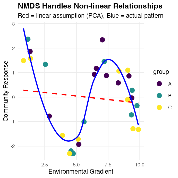
Scatterplot of a simulated sinusoidal (non-linear) relationship colored by group, with a red dashed linear fit line and a blue loess curve, showing the linear fit missing the true non-linear pattern that NMDS is robust to.

Part 4 · Running and Visualizing NMDS

NMDS in Practice

Running NMDS on Fish Communities

# Prepare species data (remove site column)
spe_matrix <- doubs_spe %>% select(-site, -reach) %>% as.matrix()
# Add small constant to avoid issues with zeros
spe_matrix <- spe_matrix + 0.1
# Run NMDS with multiple random starts
set.seed(123)
fish_nmds <- metaMDS(spe_matrix, distance = "bray",  # Bray-Curtis dissimilarity
                     k = 2,   trymax = 100)            # 2 dimensions + Maximum tries
## Run 0 stress 0.07449349 
## Run 1 stress 0.1201175 
## Run 2 stress 0.1201749 
## Run 3 stress 0.1195174 
## Run 4 stress 0.1201175 
## Run 5 stress 0.1468615 
## Run 6 stress 0.1395204 
## Run 7 stress 0.09450578 
## Run 8 stress 0.07460885 
## ... Procrustes: rmse 0.02069815  max resid 0.09861179 
## Run 9 stress 0.1273318 
## Run 10 stress 0.1200159 
## Run 11 stress 0.1273318 
## Run 12 stress 0.07449349 
## ... Procrustes: rmse 4.373445e-06  max resid 1.595028e-05 
## ... Similar to previous best
## Run 13 stress 0.09450578 
## Run 14 stress 0.140665 
## Run 15 stress 0.07459993 
## ... Procrustes: rmse 0.02014078  max resid 0.09796964 
## Run 16 stress 0.1262615 
## Run 17 stress 0.07460885 
## ... Procrustes: rmse 0.02069823  max resid 0.09861196 
## Run 18 stress 0.09134568 
## Run 19 stress 0.07460885 
## ... Procrustes: rmse 0.02069807  max resid 0.09861147 
## Run 20 stress 0.07460885 
## ... Procrustes: rmse 0.02069863  max resid 0.09861444 
## *** Best solution repeated 1 times
cat("Final stress:", round(fish_nmds$stress, 3))
## Final stress: 0.074

NMDS in Practice

  • Code Explanation:
  • fish_nmds <- metaMDS(spe_matrix, distance = "bray", # Bray-Curtis dissimilarity
    • k = 2, trymax = 100) # 2 dimensions + Maximum tries
  • metaMDS(): Main NMDS function from vegan package
    • distance = "bray": Bray-Curtis dissimilarity (best for abundances)
    • k = 2: Two dimensions for plotting
    • trymax = 100: Try 100 random starting configurations
    • Small constant added to avoid zero-distance issues
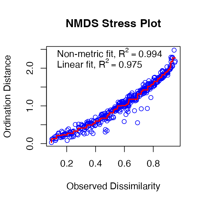
Shepard diagram (NMDS stress plot) for the fish community NMDS, showing ordination distance versus original dissimilarity closely tracking the monotonic fit line, consistent with the reported stress of 0.074.

Interpreting NMDS Output

  • Understanding the Output:

    1. Stress = 0.074 : This is “excellent”
    2. Our 2D representation preserves the original distances well
    3. Convergent solutions: Found stable solutions from multiple tries
    4. Two dimensions: Axis 1 and Axis 2 have no inherent meaning (unlike PCA components)
    5. No eigenvalues: NMDS doesn’t calculate variance explained per axis
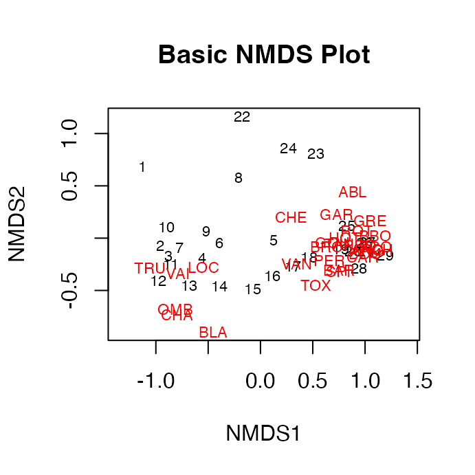
Basic NMDS ordination plot with sites plotted as text labels in 2D NMDS space, the raw base-R output before adding color-by-reach styling.

Creating Enhanced NMDS Plots

  • What the NMDS Shows:
    • Clear separation between river reaches

    • Gradient pattern from upper to lower reaches

    • Sites within each reach are more similar to each other than to other reaches
Two side-by-side NMDS ordination plots of fish community sites: one colored by river reach with confidence ellipses showing clear separation between upstream, midstream, and downstream groups; the other colored by continuous distance from source showing a smooth gradient.

Different plot using the actual hull definitions from vegan
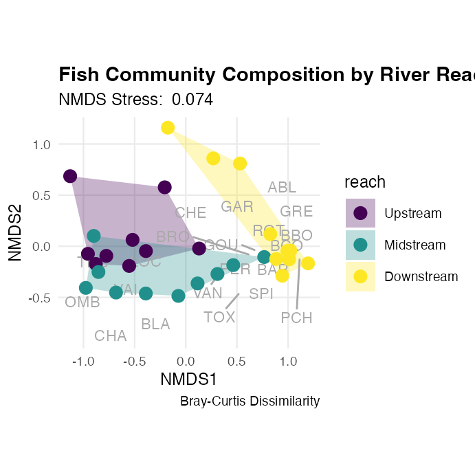
NMDS ordination plot with convex hull polygons drawn around sites in each river reach, species names plotted as grey text labels, and site points colored by reach, showing fish community composition structured along the river.

Part 5 · PERMANOVA

PERMANOVA: Testing Multivariate Differences

  • What is PERMANOVA?
    • PERMANOVA (Permutational Multivariate ANOVA):
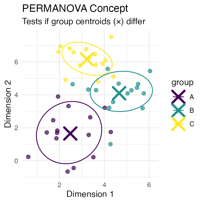
      • Purpose: Test whether groups have different multivariate centroids
      • Method: ANOVA using distance matrices instead of raw data
      • Advantage: No distributional assumptions
      • Permutation: Creates null distribution by randomly reassigning group labels
    • Think of it as:
      • Multivariate version of ANOVA

      • Uses distances between samples instead of means

      • Tests: “Are the centers of these groups different in multivariate space?” .

Scatterplot of three simulated groups with confidence ellipses and X marks showing each group's centroid, illustrating the concept PERMANOVA tests: whether group centroids differ.

How PERMANOVA Works

  • PERMANOVA Algorithm:
    1. Calculate distance matrix between all pairs of samples
    2. Calculate F-statistic based on distances:
      • Between-group sum of squares
      • Within-group sum of squares
    3. Permute group labels randomly (e.g., 999 times)
    4. Recalculate F-statistic for each permutation
    5. Compare observed F to permutation distribution
    6. P-value = proportion of permuted F ≥ observed F
  • Why permutation?
    • No assumptions about data distribution

    • Creates empirical null distribution

    • Accounts for complex dependency structures
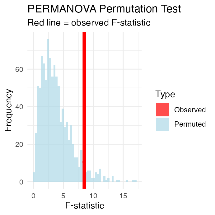
Histogram of the null distribution of F-statistics from 999 PERMANOVA permutations, with a red vertical line marking the observed F-statistic (8.5) far to the right of the null distribution.

PERMANOVA Hypotheses

  • Research Question: “Do fish communities differ significantly between river reaches?”
  • Statistical Hypotheses:
    • H₀: The centroids of fish communities are the same across all river reaches (Upper = Middle = Lower)
    • H₁: At least one river reach has a different community centroid
  • In practical terms: -
    • H₀: River position doesn’t affect community composition

    • H₁: River position significantly affects community composition
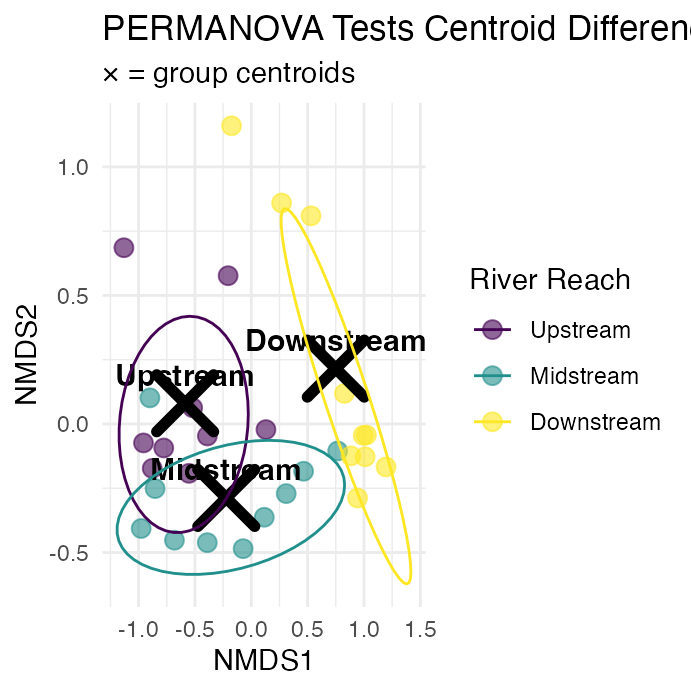
NMDS ordination plot of fish community sites colored by river reach with confidence ellipses, black X marks and text labels showing each reach's group centroid, illustrating the centroid differences PERMANOVA tests.

PERMANOVA Assumptions

  • PERMANOVA Assumptions:
  • Required:
    1. Independence: Samples are independent
    2. Exchangeability: Under H₀, observations are exchangeable between groups
    3. Homogeneity of dispersion: Groups have similar multivariate spread
  • Not required:
    • Normality or other distribution
    • Linearity
  • Checking Assumptions:
    • Use betadisper() to test homogeneity of dispersion
    • If violated, PERMANOVA is testing dispersion differences and not location differences
## Homogeneity of dispersion test p-value: 0.8037
  • vegan::betadisper() converts bray-curtis to euclidean distances to calculate distance from sample to center
  • Principal Coordinates Analysis (PCoA) - ordination for distances between samples in a low-dimensional, Euclidean space
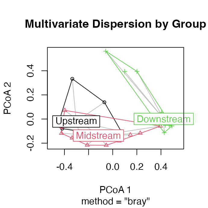
PCoA-based dispersion plot showing sites in each river reach with lines connecting each site to its group centroid, and confidence ellipses, used to check the homogeneity-of-dispersion assumption for PERMANOVA.

Running PERMANOVA

  • PERMANOVA on Fish Communities
    • Line-by-line interpretation:
      1. reach: The factor being tested (river reach)
      2. Df = 2: Degrees of freedom (3 groups - 1)
      3. SumOfSqs: Between-group sum of squares
      4. R2: Proportion of variance explained by reach
      5. F: F-statistic (ratio of between/within group variation)
      6. Pr(>F): P-value from permutation test
## Permutation test for adonis under reduced model
## Permutation: free
## Number of permutations: 999
## 
## adonis2(formula = spe_matrix ~ reach, data = doubs_env, permutations = 999, distance = "bray")
##          Df SumOfSqs      R2      F Pr(>F)    
## Model     2   2.3631 0.42634 9.6614  0.001 ***
## Residual 26   3.1798 0.57366                  
## Total    28   5.5429 1.00000                  
## ---
## Signif. codes:  0 '***' 0.001 '**' 0.01 '*' 0.05 '.' 0.1 ' ' 1
  • What this means:
    • Significant result (p < 0.001): We reject H₀

    • River reach explains substantial variation in fish communities

    • Fish communities differ significantly between river reaches

    • Very few permutations gave F ≥ observed F

Pairwise PERMANOVA Tests

  • Interpretation of Pairwise Results:
    • All pairwise comparisons are statistically significant even after Bonferroni correction

    • Upper vs Lower shows the strongest difference (highest F-statistic)

    • Downstream comparisons to up and middle explains a substantial portion of variance (R² > 0.3)

    • Biological interpretation: Fish communities change progressively down the river

##                     pairs Df SumsOfSqs   F.Model        R2 p.value p.adjusted
## 1   Upstream vs Midstream  1 0.4068962  3.434528 0.1680747   0.021      0.063
## 2  Upstream vs Downstream  1 1.8495110 15.490360 0.4767679   0.001      0.003
## 3 Midstream vs Downstream  1 1.2829784  9.972485 0.3565105   0.001      0.003
##   sig
## 1    
## 2   *
## 3   *

Visualizing PERMANOVA Results

Results:
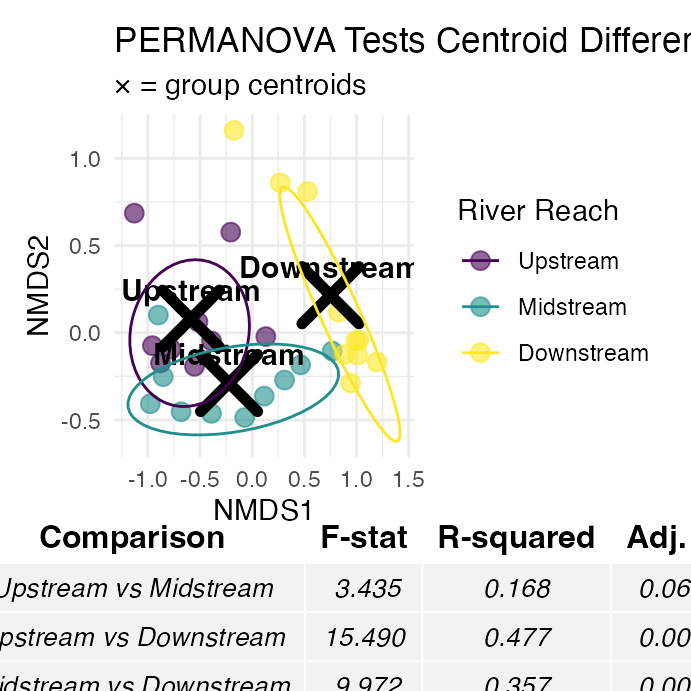
Combined figure: an NMDS plot with centroids and confidence ellipses by river reach on top, and a table of pairwise PERMANOVA comparison results (F-statistic, R-squared, adjusted p-value) below.

Part 6 · ANOSIM

ANOSIM: Analysis of Similarities

  • ANOSIM (Analysis of Similarities):
    • Purpose: are samples w/in groups are more similar than samples between groups
    • Method: Based on rank dissimilarities
    • Statistic: R-statistic ranging from -1 to +1
    • Interpretation:
      • R ≈ 1: Groups are completely separated

      • R ≈ 0: Groups are indistinguishable

      • R < 0: More dissimilarity within groups than between

  • Differences from PERMANOVA:
    • ANOSIM uses ranks of distances

    • PERMANOVA uses actual distances

    • ANOSIM is more robust but less powerful
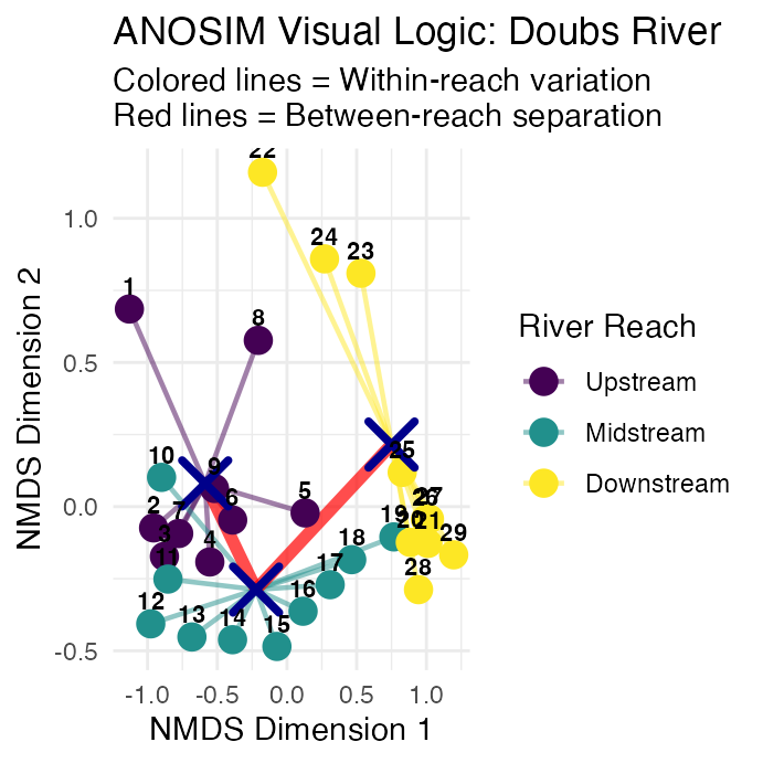
NMDS ordination plot with colored segments connecting each site to its river-reach centroid (within-group distances) and red lines connecting the reach centroids to each other (between-group distances), illustrating the logic ANOSIM tests.

How ANOSIM Works

  • ANOSIM Algorithm:
    1. Calculate dissimilarity matrix between all samples
    2. Rank all dissimilarities from smallest to largest
    3. Calculate mean rank of within-group dissimilarities (r̄w)
    4. Calculate mean rank of between-group dissimilarities (r̄b)
    5. Compute R-statistic: R = (r̄b - r̄w) / (N(N-1)/4) where N = total number of samples
    6. Permute group labels and recalculate R many times
    7. P-value = proportion of permuted R ≥ observed R
  • R-statistic interpretation:
    • R = 1: Perfect separation

    • R = 0: No separation

    • R = -1: More similar between groups than within

# Run ANOSIM
anosim_result <- anosim(spe_matrix, doubs_env$reach, 
                       distance = "bray", permutations = 999)

# Display results
anosim_result
## 
## Call:
## anosim(x = spe_matrix, grouping = doubs_env$reach, permutations = 999,      distance = "bray") 
## Dissimilarity: bray 
## 
## ANOSIM statistic R: 0.5082 
##       Significance: 0.001 
## 
## Permutation: free
## Number of permutations: 999

Running ANOSIM

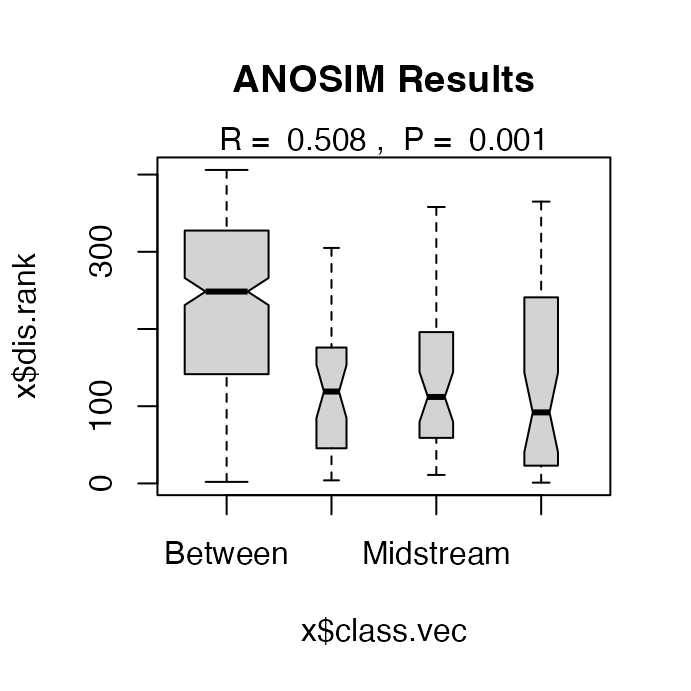
  • ANOSIM Results Interpretation:
    • R = 0.5082 : This indicates “good” separation between groups
    • **p-value = 0.001 - significant result
    • Biological meaning: Fish communities well-separated between river reaches, with communities within each reach being much more similar to each other than to communities in other reaches
  • “Within” box is clearly lower than the “Between” box
    • sites within same river reach tend to be more similar to each other (lower dissimilarity ranks) than sites in different reaches (higher dissimilarity ranks)

    • R statistic of 0.51 quantifies this separation

      • there’s clear differentiation, but with some overlap.
  • Interpreting R:

    • R = 1 - Complete separation
      • all within-group dissimilarities smaller than between-group dissimilarities
    • R > 0.75 Well separated
    • R > 0.5 Separated, but overlapping
    • R > 0.25 Barely separated
    • R ≈ 0 No difference between groups

    Boxplots of dissimilarity ranks for within-group versus between-group comparisons from the ANOSIM test, showing the within-group box clearly lower than the between-group box, consistent with an R-statistic of 0.51.

Part 7 · Comparing PERMANOVA and ANOSIM

ANOSIM vs PERMANOVA Comparison

## # A tibble: 2 × 6
##   Method    `Test Statistic` `P-value` Interpretation   `What it tests` Approach
##   <chr>     <chr>                <dbl> <chr>            <chr>           <chr>   
## 1 PERMANOVA F = 9.66             0.001 Groups have dif… Differences in… Uses ac…
## 2 ANOSIM    R = 0.508            0.001 Excellent group… Overlap betwee… Uses ra…

ANOSIM vs PERMANOVA Comparison

  • When to use which:
    • PERMANOVA:
      • More powerful for detecting differences

      • Better for complex experimental designs

      • Can handle interactions and covariates

      • Preferred for most applications

    • ANOSIM:
      • More robust to outliers
      • Simpler interpretation
      • Good for initial exploratory analysis
      • Useful when distributions are very non-normal

PERMANOVA vs ANOSIM

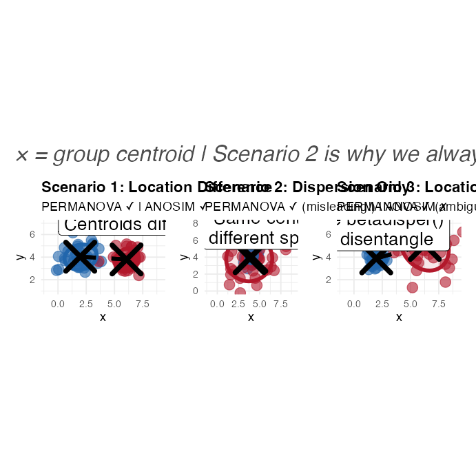
  • What’s the Difference? Three Scenarios
  • Both methods test whether groups differ, but they ask different questions:
    • PERMANOVA asks: Do the group centroids differ in location?
      • Uses actual squared distances and partitions variance like ANOVA
    • ANOSIM asks: Are within-group dissimilarities smaller than between-group?
      • Uses ranked distances to compares rank distributions

Three side-by-side scatterplots of simulated two-group data with confidence ellipses and centroid markers, illustrating three scenarios: a clear centroid difference detected by both PERMANOVA and ANOSIM, a dispersion-only difference misleadingly flagged by PERMANOVA but not ANOSIM, and a combined location-and-dispersion difference detected by both.

Scenario 2 is Key!

  • The Problem:
    • Groups A and B have the same centroid (same average community)
    • But Group B is much more variable (spread out)
    • PERMANOVA will detect this as “significant”!
  • Why?
    • PERMANOVA tests distances from points to centroids
    • More spread = larger distances = detected as “different”
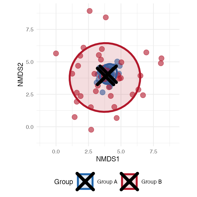
Scatterplot of two simulated groups with the same centroid but very different spread, with confidence ellipses and centroid markers, showing why PERMANOVA can misleadingly flag a 'significant' result driven only by dispersion differences.

Dispersion test for PERMANOVA

  • Solution: Always run betadisper() before interpreting PERMANOVA!
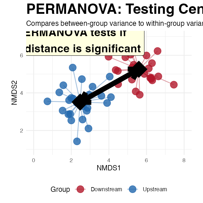
    • What PERMANOVA “Sees”

Scatterplot of two simulated groups with lines connecting each point to its group centroid and a double-headed arrow between the two centroids, illustrating that PERMANOVA tests whether the distance between group centroids is significant.

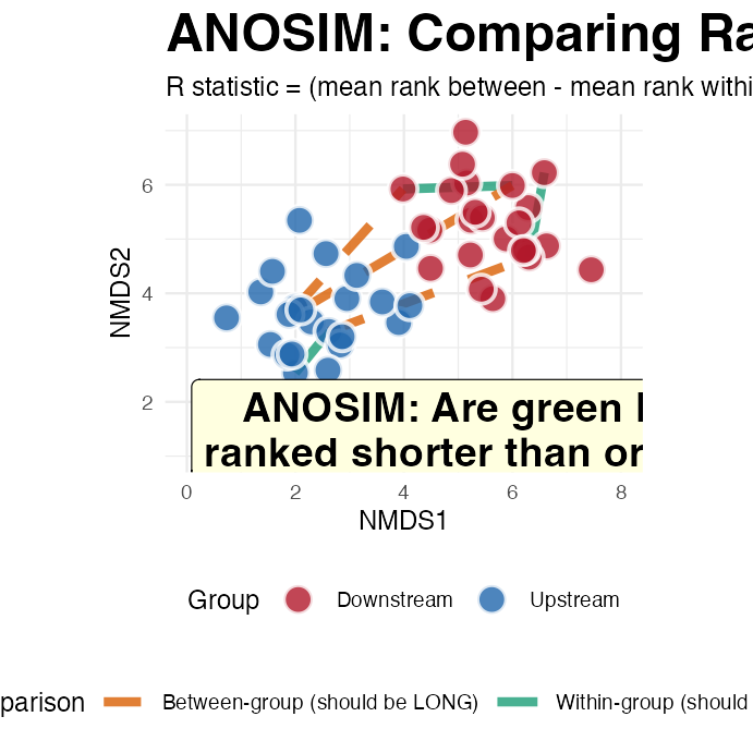
What ANOSIM “Sees”

  • This is different

Scatterplot of two simulated groups with green solid lines connecting example within-group point pairs and orange dashed lines connecting example between-group point pairs, illustrating that ANOSIM compares whether within-group distances rank shorter than between-group distances.

Side-by-Side Comparison of PCA and ANOSIM

Comparison
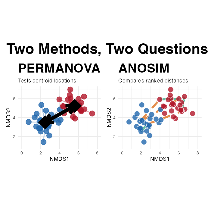
Two side-by-side scatterplots of the same simulated two-group data: the left panel shows the PERMANOVA view with centroid distances, the right panel shows the ANOSIM view with within- versus between-group distance lines.

Part 8 · Environmental Drivers and Wrap-Up

Environmental Drivers

  • Environmental Vector Results:
    • Which Environmental Variables Matter?
    • Significant variables (p < 0.05):
  • What this means:
    • variables significantly correlate w/ comm. comp
    • explain spatial arrangement of sites in NMDS
  • arrows show direction of max change for env. variables
    • Longer arrows = stronger correlations with ordination
    • Arrow direction = sites have high vs. low values of variable
  • distance from source (das) and altitude (alt) point opp. directions
    • (expected - altitude decreases as distance increases)
  • Oxygen (oxy) decreases downstream
  • BOD (dbo) increases downstream = more org. pollution
## 
## ***VECTORS
## 
##        NMDS1    NMDS2     r2 Pr(>r)    
## das  0.98098  0.19411 0.7284  0.001 ***
## alt -1.00000 -0.00057 0.5650  0.001 ***
## pen -0.61902  0.78538 0.2546  0.026 *  
## deb  0.99744 -0.07146 0.5701  0.001 ***
## pH  -0.09760 -0.99523 0.0746  0.374    
## dur  0.99967 -0.02575 0.2960  0.008 ** 
## pho  0.22860  0.97352 0.5228  0.001 ***
## nit  0.66665  0.74537 0.5200  0.001 ***
## amm  0.19902  0.98000 0.5471  0.002 ** 
## oxy -0.46402 -0.88583 0.7826  0.001 ***
## dbo  0.20211  0.97936 0.6883  0.001 ***
## ---
## Signif. codes:  0 '***' 0.001 '**' 0.01 '*' 0.05 '.' 0.1 ' ' 1
## Permutation: free
## Number of permutations: 999
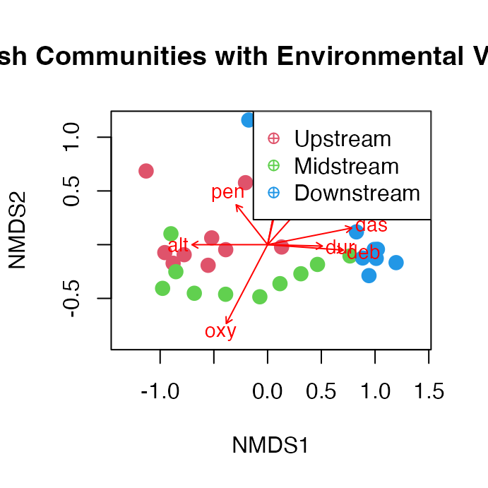
NMDS ordination plot of fish community sites colored by river reach, with red arrows overlaid showing the direction and strength of significant environmental variables (such as distance from source, oxygen, and biological oxygen demand).

Environmental Gradient Analysis

  • Key Environmental Patterns:
    • Distance from source (das): Strong correlate with community change
    • Oxygen (oxy): Decreases downstream, affects fish communities
    • Biological oxygen demand (dbo): Increases downstream (pollution indicator)
    • Altitude (alt): Decreases downstream, associated with temperature changes
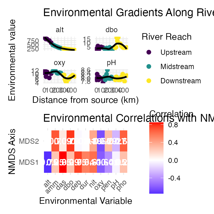
Two-panel figure: faceted scatterplots of pH, oxygen, biological oxygen demand, and altitude against distance from source with loess trend lines colored by river reach; and a correlation heatmap of the two NMDS axes against each environmental variable, with correlation values printed in each cell.

Summary and Conclusions

  • Key Findings
  • NMDS Results:
    • Stress =: Excellent representation
    • Clear gradient from upper to lower river reaches
    • Within-reach similarity greater between-reach similarity
  • PERMANOVA Results:
    • Highly significant differences between reaches (p < 0.001)
    • River reach explains substantial variance in community composition
    • All pairwise comparisons significant after correction
  • ANOSIM Results:
    • R = 0.508 p = 0.001 : Excellent separation
    • Confirms PERMANOVA findings with different approach
    • Strong within-group coherence
  • Environmental Drivers:
    • Distance from source: Primary gradient
    • Dissolved oxygen: Decreases downstream
    • Biological oxygen demand: Increases downstream
    • Multiple correlated factors drive community change
  • Biological Interpretation:
    • River continuum concept supported
    • Progressive community change from source to mouth
    • Environmental filtering shapes community assembly
    • Pollution gradient evident in lower reaches

Take-Home

  • NMDS (Non-metric Multidimensional Scaling):
    • Visualizes community dissimilarity in 2D/3D
    • Preserves rank order of distances (non-metric)
    • No distributional assumptions
    • Stress < 0.2 for acceptable solutions
    • Great for exploring ecological gradients
  • PERMANOVA (Permutational MANOVA):
    • Tests for differences in group centroids
    • Uses distance matrices, not raw data
    • No distributional assumptions
    • Can handle complex designs
    • Check dispersion homogeneity assumption
  • ANOSIM (Analysis of Similarities):
    • Tests group separation using rank distances
    • R-statistic: -1 (no separation) to +1 (complete)
    • More robust to outliers than PERMANOVA
    • Simpler but less powerful
    • Good for exploratory analysis
  • Environmental Drivers:
    • Use envfit() to correlate environment with ordination
    • Identifies which variables explain community patterns
    • Helps understand ecological mechanisms
    • Essential for management implications