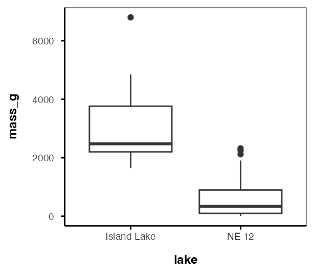
Lecture: Non-Parametric T-Tests

Rank-based tests

Bill Perry

Where We Left Off

A brief review:

• Hypotheses
• One- and two-sided t-tests
• One-sample, two-sample, and paired t-tests — and how much more the paired test got out of the same four trees
• Assumptions of parametric tests
• What next — when assumptions fail!
  • we will always cover parametric tests first
  • then non-parametric approaches
  • later, other approaches use the appropriate underlying distribution when it isn’t normal, but Poisson or other

Note

✅ Key idea from last lecture

A t-test’s p-value is only trustworthy if its assumptions hold. Today is about how to tell whether they do — and what to do when they don’t.

Photo comparing needle length and bundle count across six pine species (Pinus ponderosa, nigra, resinosa, strobus, sylvestris, banksiana).

Warning

⚠️ The trap we’re walking into first

It is tempting to treat non-parametric tests as the “safe” option you can always fall back on. We are going to start by showing why that instinct is wrong.

Today’s Overview

Today runs in two halves, and the order matters:

1. Our own pine needles first. We check the assumptions on the data you collected, find that they hold, measure how big the effect actually was with Cohen’s d, and then run the non-parametric tests anyway — to see exactly what they cost.
2. Then the lake trout. A dataset where the assumptions are genuinely, badly broken — which is where robust tests, rank-based tests, and permutation tests earn their keep.

Note

✅ The question behind today

Not “which test is safest?” but “which test does this data deserve?”

Photo comparing needle length and bundle count across six pine species (Pinus ponderosa, nigra, resinosa, strobus, sylvestris, banksiana).

Illustration of a lake trout in profile, showing its mottled brown-and-cream coloring and forked tail, the species whose weight and length data are used in the second half of this lecture.

Part 1 · Start With Our Own Data

Our pine needles, where we left them

library(tidyverse)
library(janitor)
library(car)          # leveneTest()
library(patchwork)
library(perm)         # permutation tests
library(effectsize)   # cohens_d()

source("themes_functions/r_themes_and_functions.R")

pine_df <- read_csv("data/pine_data.csv")

# same two-stage summary as last week: one value per tree per side
p_df <- pine_df %>%
  group_by(team, side) %>%
  summarise(needle_length_mm = mean(needle_length_mm, na.rm = TRUE),
            .groups = "drop")

p_wide_df <- p_df %>%
  pivot_wider(names_from = side, values_from = needle_length_mm)

p_wide_df

# A tibble: 4 × 3
  team       shady sunny
  <chr>      <dbl> <dbl>
1 botany      16.1  17.3
2 grace_jace  15.4  15.5
3 one         13.2  14.2
4 waterbugs   11.7  13.8

📥 Pine needle data 📥 Lake trout data 📥 Sagebrush cricket data

📥 Tools script 📥 Script skeleton

Note

✅ Reminder

4 teams, 4 trees, both sides of each tree. The data are paired by design.

Last week these four trees gave us:

Comparison	p
Unpaired two-sample t	0.425
Paired t	0.072

Note

✅ Same two tools as last week

source() gives you theme_regular() and summary_stats() again. Nothing new to learn.

Do our assumptions actually hold?

Note

🔮 Predict first: Before we run anything — do you expect needle length to be normally distributed with equal variance on the two sides of a tree? Commit to an answer.

Before reaching for anything non-parametric, we have to establish that we need it. Same two checks as last week.

# normality, one side at a time -- all 32 needles per side
shapiro.test(pine_df$needle_length_mm[pine_df$side == "sunny"])

    Shapiro-Wilk normality test

data:  pine_df$needle_length_mm[pine_df$side == "sunny"]
W = 0.96105, p-value = 0.2934

shapiro.test(pine_df$needle_length_mm[pine_df$side == "shady"])

    Shapiro-Wilk normality test

data:  pine_df$needle_length_mm[pine_df$side == "shady"]
W = 0.98213, p-value = 0.8586

# equal variance
leveneTest(needle_length_mm ~ factor(side), data = pine_df)

Levene's Test for Homogeneity of Variance (center = median)
      Df F value Pr(>F)
group  1   2e-04 0.9887
      62               

Important

⚠️ Everything passes

Check	p
Shapiro-Wilk, sunny	0.29
Shapiro-Wilk, shady	0.86
Levene’s	0.99

Remember the direction of these tests: H₀ is that the assumption holds. A large p means we have no evidence against it.

There is nothing wrong with this data. The paired t-test we ran last week was entitled to every bit of its p = 0.072.

Tip

🖐 So why are we here?

Because “my data are fine” is a conclusion you have to earn, not assume — and because plenty of students would have reached for a rank test anyway, thinking it was the cautious choice. Let’s find out what that caution would have cost.

Effect Size — How Big, Not Just Whether

Our paired t-test gave p = 0.072. The usual reflex is to call that “not significant” and stop.

But p never told us the one thing a reader actually wants to know: how much shorter are shady needles? A p-value answers “could this be noise?” — not “does this matter?”

Cohen’s d answers the second question. It is the difference between the groups expressed in standard deviations, so it has no units and can be compared across studies:

\[d = \frac{\bar{x}_1 - \bar{x}_2}{s}\]

For a paired design the difference is the paired difference, and s is the standard deviation of those differences:

diffs <- p_wide_df$shady - p_wide_df$sunny

mean(diffs) / sd(diffs)     # Cohen's d, by hand

[1] -1.361371

Note

✅ Read the formula out loud

“The shady side averaged 1.36 standard deviations below the sunny side.”

That sentence stands on its own. It does not depend on how many trees we sampled, and it would mean the same thing to someone measuring a different pine species in a different forest.

Tip

🖐 Cohen’s rough conventions

|d|	Label
0.2	small
0.5	medium
0.8	large

Ours is 1.36. These are rules of thumb, not laws — what counts as “large” is a question about pine trees, not about statistics.

Why We Report It — What d Tells Us That p Could Not

Here is the relationship that explains everything:

\[t = d \times \sqrt{n}\]

2.7227 / sqrt(4)      # our t statistic, over root n

[1] 1.36135

The t-statistic is the effect size multiplied by the square root of your sample size. So a p-value confounds two completely different things: how big the effect is, and how hard you looked.

• A huge effect with n = 4 → large p. That is us.
• A trivial effect with n = 10,000 → tiny p, and no biological meaning at all.

Effect size separates them. That is why journals, and every reporting guideline written in the last twenty years, ask for it alongside the p-value.

library(effectsize)

cohens_d(p_wide_df$shady,
         p_wide_df$sunny,
         paired = TRUE)

Cohen's d |        95% CI
-------------------------
-1.36     | [-2.74, 0.10]

Important

⚠️ Look at that confidence interval: [-2.74, 0.10]

This is the honest summary of our four trees: the effect is probably large and probably negative, but with n = 4 we cannot rule out zero.

Notice that the CI crossing zero is the same fact as p > 0.05 — but it says it far more usefully. “No significant difference” sounds like we found nothing. “d = -1.36, CI [-2.74, 0.10]” says we found a large effect we could not pin down, which is a completely different message to a reader, and the correct one.

Tip

🖐 Where this goes next

Effect size is the input to a power analysis — given d, how many trees would we have needed? That is next week’s lecture.

Ranks, in one slide

Every non-parametric test today works the same way: throw away the measurements, keep only their order.

p_df %>%
  mutate(rank = rank(needle_length_mm)) %>%
  arrange(rank)

# A tibble: 8 × 4
  team       side  needle_length_mm  rank
  <chr>      <chr>            <dbl> <dbl>
1 waterbugs  shady             11.7     1
2 one        shady             13.2     2
3 waterbugs  sunny             13.8     3
4 one        sunny             14.2     4
5 grace_jace shady             15.4     5
6 grace_jace sunny             15.5     6
7 botany     shady             16.1     7
8 botany     sunny             17.3     8

Note

✅ What just happened

The shortest tree-side average became rank 1, the longest rank 8. A needle that was 4 mm longer than its neighbour and one that was 0.1 mm longer are now exactly one rank apart.

That is the whole trade. You become immune to outliers and to any weird distribution — and in exchange you give up the magnitudes.

A rank-based test then asks: are the ranks of one group systematically higher than the other’s?

Tip

🖐 Watch for the statistic

Rank tests report W (Mann-Whitney) or V (signed-rank), never t. If you see a W, you are reading rank-based output.

Running both rank-based tests

# Unpaired: Mann-Whitney U  (the t-test's two-sample partner)
wilcox.test(needle_length_mm ~ side, data = p_df)

    Wilcoxon rank sum exact test

data:  needle_length_mm by side
W = 5, p-value = 0.4857
alternative hypothesis: true location shift is not equal to 0

# Paired: Wilcoxon signed-rank  (the paired t-test's partner)
wilcox.test(p_wide_df$shady, p_wide_df$sunny, paired = TRUE)

    Wilcoxon signed rank exact test

data:  p_wide_df$shady and p_wide_df$sunny
V = 0, p-value = 0.125
alternative hypothesis: true location shift is not equal to 0

Tip

🖐 Notice V = 0

The signed-rank statistic is zero — meaning every single tree moved in the same direction. There is no arrangement of these four trees that would look more consistent.

Notice too that R says “exact test” for both. With no tied values it enumerates every possible arrangement rather than approximating. Hold on to that word — the next slide explains why it matters.

Same answer, less power

Comparison	Parametric	Non-parametric
Unpaired (2 groups)	t-test p = 0.425	Mann-Whitney p = 0.486
Paired (4 trees)	paired t p = 0.072	signed-rank p = 0.125

Both methods tell the same story:

• the unpaired comparison finds nothing
• the paired comparison is far more sensitive
• the direction is identical — shady needles shorter

But the rank test costs you. In both rows the non-parametric p-value is larger. That is the price of throwing away the actual measurements and keeping only their order — and we paid it on data that never needed it.

Important

⚠️ At n = 4, the signed-rank test hits a wall

With 4 pairs there are only 2⁴ = 16 possible arrangements of plus and minus signs. The most extreme possible result — all four the same way, which is exactly what we got — has a two-sided p of 2/16 = 0.125.

So with four trees, a Wilcoxon signed-rank test can never return a p-value below 0.125, no matter how enormous the effect.

2 / 2^4     # smallest possible two-sided p, 4 pairs

[1] 0.125

The test did not fail to find our effect. It was arithmetically incapable of declaring it significant.

What that means in practice

• Non-parametric tests are the right call when normality is genuinely broken and cannot be fixed
• But they are not free, and they are not a safe default
• At small n they can be so blunt that no result could ever reach significance — check the floor before you run one

Note

✅ Key idea

Choose the test that matches your data’s distribution, not the one that feels safest. For our four trees, the parametric paired t-test — whose assumptions we just checked and could not reject — is the more honest and more informative choice.

Tip

🖐 Try it yourself

How many pairs would you need before a signed-rank test could reach p < 0.05?

2 / 2^5    # 5 pairs
2 / 2^6    # 6 pairs

Warning

⚠️ Where we go next

We have now seen what these tests cost. What we have not seen is what they buy you — because nothing about the pine data was broken.

For that we need a dataset that is a genuine mess.

Part 2 · A Dataset Where the Assumptions Really Do Fail

Meet the lake trout

lt_df <- read_csv("data/lake_trout.csv")

lt_df %>% group_by(lake) %>% reframe(summary_stats(mass_g))

# A tibble: 6 × 7
  lake            n  mean    sd    se ci_lower ci_upper
  <chr>       <int> <dbl> <dbl> <dbl>    <dbl>    <dbl>
1 I8             91  857.  727.  76.2     705.    1008.
2 Island Lake    10 3165  1617. 511.     2008.    4322.
3 N 01          674  659.  395.  15.2     629.     689.
4 NE 12         322  534.  520.  29.0     477.     591.
5 NE 14         139  848.  508.  43.1     763.     933.
6 Toolik        249  518.  373.  23.6     471.     564.

📥 Lake trout data

Tip

🖐 Notice the design

Six lakes of trout: sampling_site, species, length_mm, mass_g, lake.

Everything from here on uses mass_g. Look hard at the n and sd columns for NE 12 and Island Lake — 322 fish against 10, and very different spreads.

That imbalance is the rest of the lecture. Where the pine data was clean, this is everything that can go wrong at once.

Part 3 · Assumptions of Parametric Tests

Parametric vs. Non-Parametric Tests

T-tests are parametric tests.

• Parametric tests:
  • specify/assume the probability distribution the parameters came from
  • basic assumptions of parametric t-tests: random sampling, normality, equal variance (or Welch’s t-test), no outliers
• Non-parametric tests: no assumption about the probability distribution/normality
  • Mukasa et al. 2021, DOI: 10.4236/ojbm.2021.93081

Note

📖 Reference

Whitlock & Schluter, Analysis of Biological Data, Ch. 13 — Handling Violations of Assumptions, is the core reference for this whole lecture.

Flowchart of hypothesis tests branching into parametric and nonparametric tests, each split into one-sample and two-sample (independent vs. paired) tests, listing specific tests under each branch (e.g., t test and z test under parametric one-sample; Mann-Whitney and Wilcoxon under nonparametric two-sample).

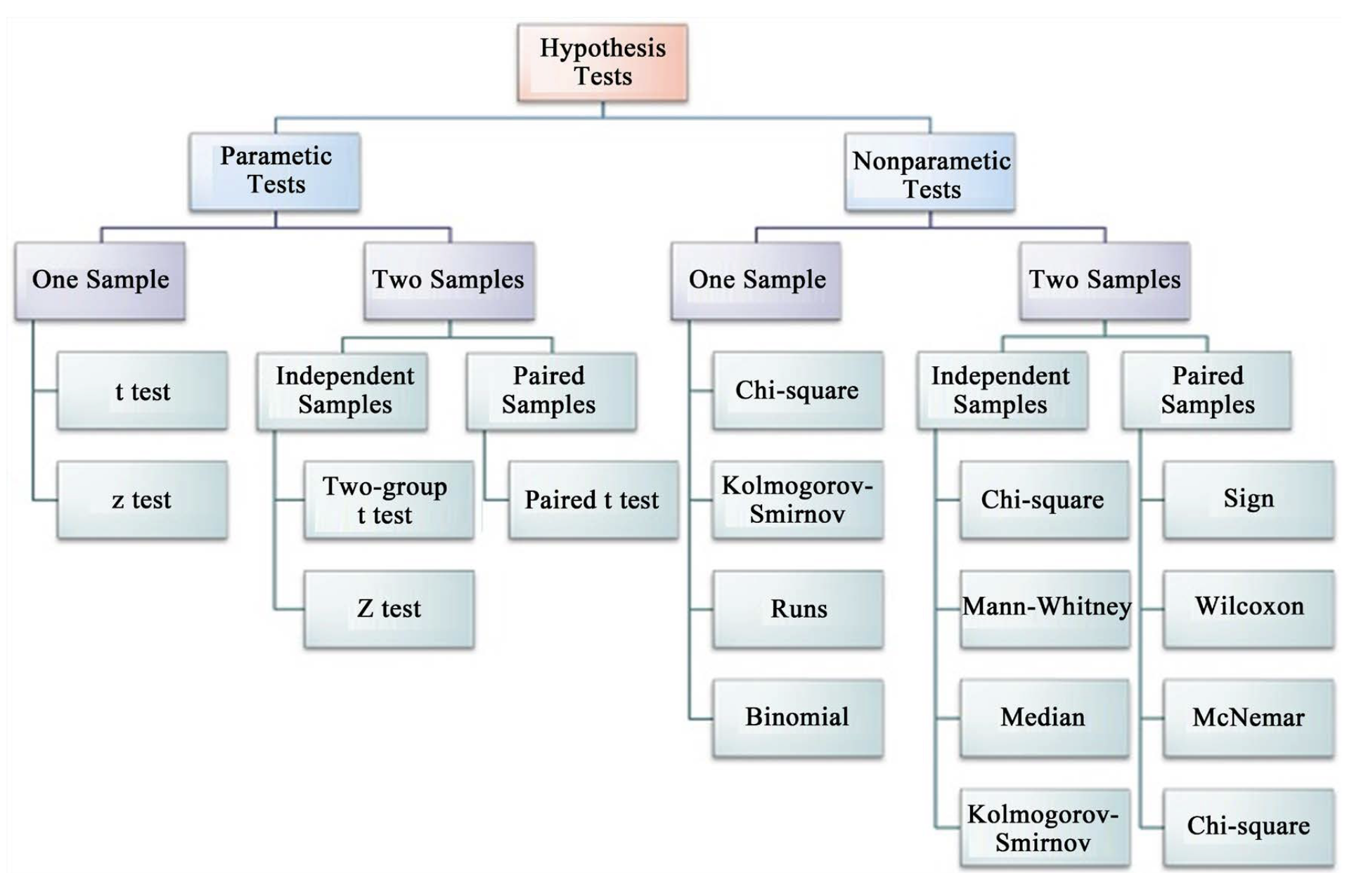
Assumptions of Parametric Tests — Overview

• If a parametric test’s assumptions are violated, the test becomes unreliable
• This is because the test statistic may no longer follow the distribution it’s supposed to
• Most parametric tests are robust to mild/moderate violations of normality

Three probability density curves for a right-skewed distribution family at different sigma values (0.25, 0.5, 1) with mu = 0, showing how larger sigma produces a flatter, more spread-out, and less peaked skewed curve.

Assumptions — Random Sampling

Basic assumptions of parametric t-tests: random sampling, normality, equal variance, no outliers.

Random sampling:

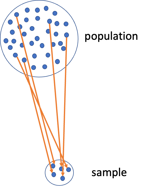
• samples are randomly collected from populations; part of experimental design
• necessary for sample → population inference

Diagram of a large circle labeled ‘population’ full of dots, with orange arrows showing a subset being drawn down into a small circle labeled ‘sample’, illustrating random sampling from a population.

Assumptions — Normality Testing

Note

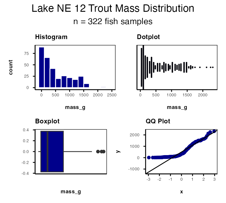
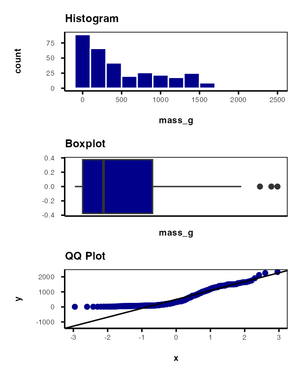
🔮 Predict first: We’re about to look at histogram, dotplot, boxplot, and QQ-plot views of the same NE 12 mass data. Which of the four do you expect to be most convincing about normality?

Let’s test normality for one lake — NE 12 — as if we were going to run a one-sample t-test. We need a new data frame with only NE 12 data, called ne12_data.

Normality: samples from a normally distributed population

• Graphical tests: histograms, dotplots, boxplots, QQ-plots
• “Formal” tests: Shapiro-Wilk test — sometimes not useful

Shapiro-Wilk Test for Normality

H₀ is that the data ARE normally distributed — so a small p-value rejects normality.

• Graphical tests: histograms, dotplots, boxplots, QQ-plots
• “Formal” tests: Shapiro-Wilk — sometimes not useful

shapiro.test(ne12_data$mass_g)

    Shapiro-Wilk normality test

data:  ne12_data$mass_g
W = 0.85148, p-value < 2.2e-16

Warning

⚠️ p prints as < 2.2e-16

That is R telling you the p-value is smaller than it will bother to print. Not a borderline call — NE 12 mass is strongly non-normal, exactly as the histogram and QQ-plot showed. This is the case the rest of the lecture is for.

Testing the Equal Variance Assumption

Equal variance: samples are from populations with a similar degree of variability.

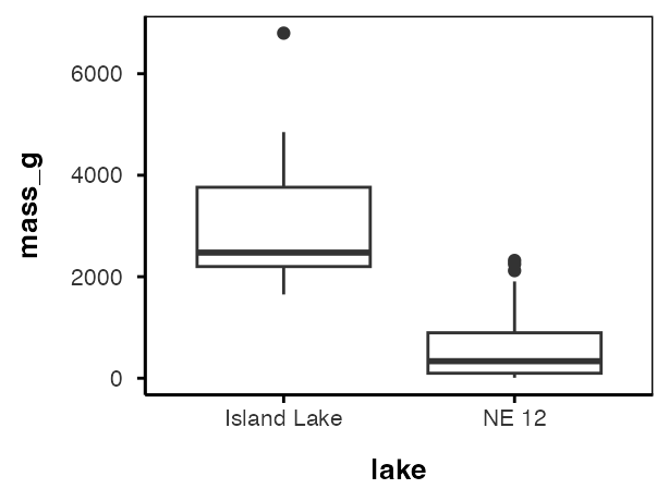
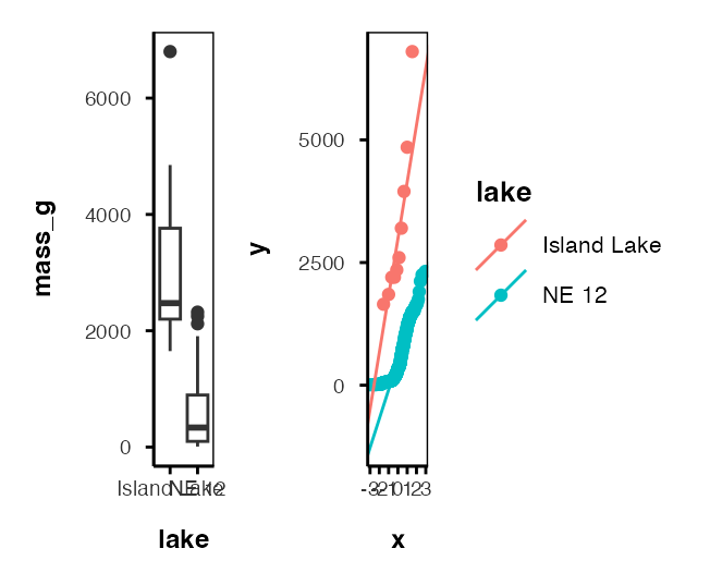
Equal variance is about two groups, so here we bring in the comparison we will use for the rest of the lecture: NE 12 vs. Island Lake.

• Graphical test: boxplots
• Formal test: Levene’s test — H₀ is “the variances are equal,” so you want p > 0.05

isl_ne12_df <- lt_df %>%
  filter(lake %in% c("NE 12", "Island Lake")) %>%
  filter(!is.na(mass_g))

isl_ne12_df %>%
  ggplot(aes(lake, mass_g)) +
  geom_boxplot() +
  theme_regular(base_size = 10)

leveneTest(mass_g ~ factor(lake), data = isl_ne12_df)

Levene's Test for Homogeneity of Variance (center = median)
       Df F value    Pr(>F)    
group   1  25.997 5.775e-07 ***
      330                      
---
Signif. codes:  0 '***' 0.001 '**' 0.01 '*' 0.05 '.' 0.1 ' ' 1

p is far below 0.05 — the variances are not equal.

Testing for Outliers

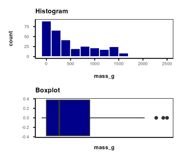
No outliers: no “extreme” values very different from the rest of the sample.

• Graphical tests: boxplots, histograms
• “Formal tests”: Grubbs’ test — no one really does this

Warning

⚠️ Watch out!

Outliers are a problem for non-parametric tests as well — switching to a rank-based test doesn’t make an outlier stop mattering.

Part 4 · When Assumptions Fail

Alternative Tests When Assumptions Fail

What if t-test assumptions fail? Alternative tests, with more relaxed assumptions, are available. In which case would you use each?

• Welch’s t-test: distribution normal but variance unequal
• Mann-Whitney-Wilcoxon test: distribution not normal and/or outliers present (but both groups should still have similar distributions and ~equal variance)
• Permutation test for two samples: distribution not normal (but both groups should still have similar distributions and ~equal variance)

Understanding QQ-Plots

QQ-plots: a tool for assessing normality.

• On x: theoretical quantiles from a standard normal distribution
• On y: ordered sample values
• Deviation from normal can be detected as deviation from a straight line

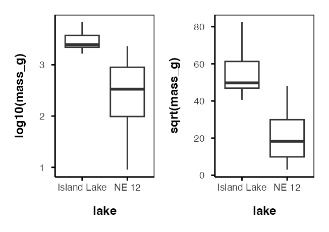
Data Transformations

In some cases, data can be mathematically “transformed” to meet the assumptions of parametric tests. This usually involves:

• log₁₀ transformations
• square root transformations
• and many others

log_box_plot <- isl_ne12_df %>%
  ggplot(aes(lake, log10(mass_g))) +
  geom_boxplot() +
  theme_regular(base_size = 9)

ne12_island_box_plot + log_box_plot

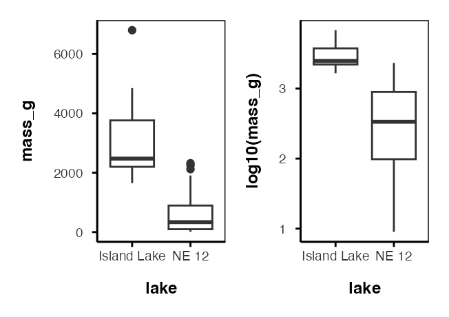
The log scale pulls the two spreads much closer together — but it does not fix them completely. Levene’s test on log10(mass_g) is still significant.

Reference chart of six common data transformations (square root, logarithm, inverse, and their ‘reflect and’ variants for left-skewed data), each shown as a small curve with its transformation formula, used to pick a transformation that matches a variable’s skew shape.

source

Data Transformations — Why Log?

Log isn’t a trick you try at random — it fixes a specific shape of problem:

• Right-skewed data (a long tail of large values) → log10(x)
• Effects that are multiplicative rather than additive (doubling a value, not adding a fixed amount) → log10(x)
• Ratio-scale ecological measurements — mass, concentration, population size, area — are almost always multiplicative

Note

✅ The mechanism, in one line

A trout that is twice as heavy as another isn’t “500 g more” — it’s “2×.” Log turns that multiplicative relationship into an additive one, which is what a t-test’s equal-spread assumption expects. It compresses the right tail: 100 g → 1000 g and 1000 g → 10,000 g become the same distance, one log unit.

Data Transformations — Beyond Log

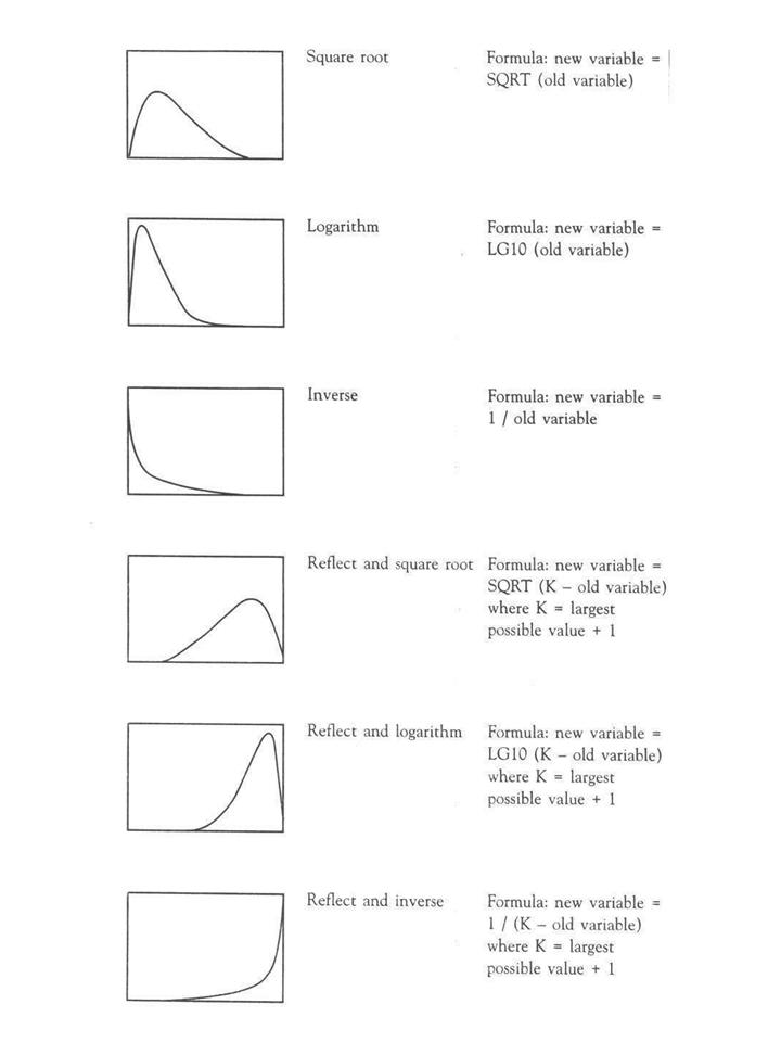
Log is the one you will reach for most in ecology, but match the transform to the shape of the problem:

Transformation	Use when…
log10(x)	right-skewed, multiplicative, ratio-scale data (mass, concentration, abundance)
sqrt(x)	count data, moderate right skew (Poisson-like variance)
asin(sqrt(x))	proportions or percentages bounded 0–1
1/x	rates, or extreme right skew that log doesn’t fix
Box-Cox	no obvious transform works — let the data pick the power

None of these are guaranteed to work. You check afterward, every time — that’s Part 5 of the worksheet, and it’s the whole point of the take-home.

sqrt_box_plot <- isl_ne12_df %>%
  ggplot(aes(lake, sqrt(mass_g))) +
  geom_boxplot() +
  theme_regular(base_size = 9)

log_box_plot + sqrt_box_plot

sqrt() narrows the spread less than log10() did here — this skew behaves more like a multiplicative effect than a count.

A Transformation Can Fix One Problem, Not the Other

leveneTest(log10(mass_g) ~ factor(lake), data = isl_ne12_df)

Levene's Test for Homogeneity of Variance (center = median)
       Df F value    Pr(>F)    
group   1   11.77 0.0006784 ***
      330                      
---
Signif. codes:  0 '***' 0.001 '**' 0.01 '*' 0.05 '.' 0.1 ' ' 1

Compare that to the Levene’s result on raw mass_g a few slides back — both fail. Normality improved with the log transform. Equal variance did not. Checking a transformation is not one pass/fail box — you re-test every assumption, separately, on the transformed variable.

Important

⚠️ This is the take-home’s whole trap

The sagebrush cricket data works the same way: a transformation can help one assumption without rescuing the other. There is no single “correct” test hiding in the data — there’s a best-justified one. Check every assumption on the raw data, then again on any transformed version, before you decide.

Part 5 · Welch’s T-Test — a One-Slide Refresher

Welch’s t-Test — why it exists, in one number

You met Welch’s last week: same t-statistic idea, separate variance estimates, fractional degrees of freedom. Nothing new to learn. What is new is this dataset, which shows you why it matters.

# Student's -- assumes equal variances
t.test(mass_g ~ lake, data = isl_ne12_df, var.equal = TRUE)

    Two Sample t-test

data:  mass_g by lake
t = 14.181, df = 330, p-value < 2.2e-16
alternative hypothesis: true difference in means between group Island Lake and group NE 12 is not equal to 0
95 percent confidence interval:
 2266.304 2996.360
sample estimates:
mean in group Island Lake       mean in group NE 12 
                3165.0000                  533.6677 

# Welch's -- does not
t.test(mass_g ~ lake, data = isl_ne12_df, var.equal = FALSE)

    Welch Two Sample t-test

data:  mass_g by lake
t = 5.1368, df = 9.0578, p-value = 0.0006016
alternative hypothesis: true difference in means between group Island Lake and group NE 12 is not equal to 0
95 percent confidence interval:
 1473.676 3788.989
sample estimates:
mean in group Island Lake       mean in group NE 12 
                3165.0000                  533.6677 

Important

⚠️ Same data. Same means. Sixty orders of magnitude apart.

	t	df	p
Student’s	14.18	330	5.7 × 10⁻³⁶
Welch’s	5.14	9.06	0.0006

(R only prints < 2.2e-16 for the first one — that is the smallest number it will show you. The true value is 5.7 × 10⁻³⁶.)

Look at the df. Student’s pooled 322 Island-sized fish with 10 NE 12-sized ones and claimed 330 degrees of freedom. Welch’s looked at the same data and said: you really only have about 9.

Both still reject H₀ — but Student’s was never entitled to that much confidence. With n = 322 vs 10 and Levene’s p ≈ 6 × 10⁻⁷, the pooled variance is meaningless.

Tip

🖐 The rule

Unequal n and unequal variance is exactly the combination Welch’s was built for. When in doubt, var.equal = FALSE is the safer default — it costs you almost nothing when variances really are equal.

Part 6 · Rank-Based Tests

Rank-Based Tests — now on data that needs them

Same two tests you ran on the pine needles in Part 1 — ranks instead of measurements, no assumption about the distribution.

• Ranks of data: observations are assigned ranks; sums (and signs, for paired tests) of ranks for groups are compared
• Mann-Whitney U test — common alternative to the independent-samples t-test
• Wilcoxon signed-rank test — alternative to the paired t-test
• Assumptions: similar distributions for groups, equal variance
• Less power than parametric tests
• Best when normality can’t be met by transformation (weird distribution) or there are large outliers

Note

✅ The difference from Part 1

On the pine needles the rank test was a cost — we gave up power on data that was already well behaved.

Here, NE 12 mass is non-normal at p < 2.2 × 10⁻¹⁶ and full of outliers. There is nothing to give up. This is the case the test was built for.

Note

📖 Reference

Whitlock & Schluter, Ch. 13, covers the Mann-Whitney U test and Wilcoxon signed-rank test as the standard rank-based alternatives.

Mann-Whitney U Test Results

wilcox_test_result <- wilcox.test(mass_g ~ lake, data = isl_ne12_df)

wilcox_test_result

    Wilcoxon rank sum test with continuity correction

data:  mass_g by lake
W = 3205.5, p-value = 9.506e-08
alternative hypothesis: true location shift is not equal to 0

Tip

🖐 W again, and no “exact” this time

The statistic is W, not t — rank-based output, as in Part 1.

But notice what R doesn’t say: with 332 fish and plenty of tied masses it cannot enumerate every arrangement, so this is the normal approximation, not an exact test. At this sample size that is fine — the floor problem that crippled our four trees does not exist here.

Part 7 · Permutation Tests

Permutation Tests — Concept

• Permutation tests are based on resampling: reshuffling the original data
• Resampling allows parameter estimation when the distribution is unknown, including SEs and CIs of statistics (means, medians)
• A common approach is the bootstrap: resample with replacement many times, recalculate sample stats
• We use the perm package
• H₀: µ_A = µ_B, Hₐ: µ_A ≠ µ_B
• Calculates the difference Δ in means between two groups

Permutation Tests — Method

• Randomly reshuffle observations between groups (keeping n₍NE 12₎ = 322 and n₍Island₎ = 10), calculate Δ
• Repeat > 1,000 times
• Record the proportion of the differences in means as extreme as (or more extreme than) observed
• This is equivalent to a p-value, and can be used in the “traditional” hypothesis-testing framework

Tip

🖐 For a graphical explanation

jwilber.me/permutationtest

Permutation Test Implementation

In R, using the perm package. Assumptions: both groups have a similar distribution; equal variance.

library(perm)

# Balance the design: take 10 NE 12 fish, keep all of Island Lake
set.seed(123)
perm_df <- bind_rows(
  isl_ne12_df %>%
    filter(lake == "NE 12") %>%
    slice_sample(n = 10),
  isl_ne12_df %>%
    filter(lake == "Island Lake")
)

# The difference the test is about
perm_df %>% group_by(lake) %>% reframe(summary_stats(mass_g))

# A tibble: 2 × 7
  lake            n  mean    sd    se ci_lower ci_upper
  <chr>       <int> <dbl> <dbl> <dbl>    <dbl>    <dbl>
1 Island Lake    10 3165  1617.  511.    2008.    4322.
2 NE 12          10  645.  538.  170.     260.    1030.

permTS(mass_g ~ lake,
       data = perm_df,
       alternative = "two.sided",
       method = "exact.mc",
       control = permControl(nmc = 10000))

    Exact Permutation Test Estimated by Monte Carlo

data:  mass_g by lake
p-value = 2e-04
alternative hypothesis: true mean lake=Island Lake - mean lake=NE 12 is not equal to 0
sample estimates:
mean lake=Island Lake - mean lake=NE 12 
                                 2519.9 

p-value estimated from 10000 Monte Carlo replications
99 percent confidence interval on p-value:
 0.000000000 0.001059383 

Part 8 · Summary

Summary — Testing Assumptions

Key assumptions:

• Random sampling — samples are randomly collected from populations
• Normality — data follows a normal distribution
• Equal variance — samples come from populations with similar variability
• No outliers — no extreme values that can skew results

Note

Assessing assumptions

• Key to do every time
• Should be acknowledged in the manuscript

Summary — Effect Size

Always report an effect size next to your p-value.

• Cohen’s d = the difference between groups, in standard deviations — unitless, and comparable across studies
• t = d × √n, so a p-value confounds how big the effect is with how hard you looked
• A confidence interval on d says what a bare “n.s.” never can: whether you found nothing, or found something you could not pin down
• Effect size is also the input to a power analysis — next week

Note

✅ On our four trees

Paired d = −1.36, CI [−2.74, 0.10], p = 0.072. A large effect, imprecisely measured. Reporting only “p = 0.072, n.s.” would have thrown that away.

Tip

🖐 In a results sentence

Needles on the shady side were 1.09 mm shorter than on the sunny side (paired t₃ = −2.72, p = 0.072, d = −1.36, 95% CI [−2.74, 0.10]).

Every number there does work the others cannot.

Summary — Data Transformations

When assumptions aren’t met, transformations may help normalize data:

• Log transformation: log10(x) — useful for right-skewed data, multiplicative effects
• Square root: sqrt(x) — useful for count data, moderately right-skewed distributions
• Box-Cox: a more flexible family of power transformations
• More specialized transformations exist, especially for percentages or proportions

Tip

🖐 Recall

We saw log10() shrink the gap between the NE 12 and Island Lake boxplots earlier — that’s the transformation working.

Summary — Parametric Test Options

1. Standard t-test

Strengths:

• High statistical power when assumptions are met
• Well understood and widely accepted

Weaknesses:

• Sensitive to violations of normality, equal variance
• Heavily influenced by outliers

2. Welch’s t-test

Covered in full in the T-Tests lecture; the one-slide refresher in Part 5 is all we needed today.

• Robust to unequal variances and unequal n — which is exactly our NE 12 vs. Island Lake case
• Still parametric: it fixes the variance assumption, not the normality one
• Costs almost nothing when variances really are equal, so it is a safe default
• On these data it moved df from 330 to 9.06 — that is the whole story

Summary — Non-Parametric Options

3. Mann-Whitney-Wilcoxon test

Strengths:

• Non-parametric: doesn’t assume normal distribution
• Robust against outliers
• Works with ordinal data

Weaknesses:

• Less statistical power than parametric tests
• Still assumes similar distributions and approximately equal variance
• Tests median differences rather than mean differences
• At small n there is a hard floor on the p-value — with 4 pairs a signed-rank test cannot go below 0.125 (see Part 1)

4. Permutation tests

Strengths:

• Distribution-free: doesn’t assume a specific distribution
• Can be applied to many types of test statistics
• Valid at small n — the p-value is exact, not an approximation
• Directly estimates p-values through resampling

Weaknesses:

• Computationally intensive
• Assumes exchangeability under the null hypothesis
• Requires similar distributions and equal variance
• Hits the same small-n floor as the rank tests — being exact is not the same as being powerful, because there are only so many ways to rearrange 8 numbers

Key Takeaway

Statistical tests have different strengths and assumptions. The choice should be guided by your data’s characteristics, not just convenience.

Always visualize your data before deciding on the appropriate test.

Note

✅ Key idea

Standard t-test → Welch’s → Mann-Whitney/Permutation isn’t a strict ladder of “better” tests — each answers a slightly different question (means vs. medians) under different assumptions. Pick based on what your data actually looks like.

Looking Ahead — The Take-Home

Part 8 of the worksheet (sagebrush crickets, due before Study Design & Sampling) hands you a new dataset and asks you to run the whole decision process from today:

1. Check normality and equal variance on the raw data
2. Try a transformation if the raw data doesn’t pass
3. Check normality and equal variance again, on the transformed data — don’t assume it worked
4. Pick a test, justify the pick, and report it properly

There is no lecture slide that tells you the answer this time.

Tip

🖐 Remember from today

log10() fixed normality for the lake trout but not equal variance. Expect the crickets to behave similarly — a transformation earning partial credit is a completely normal outcome, not a sign you did something wrong.