Lecture: Review

Course review

Bill Perry

Lecture 19: Introduction to Logistic Regression

What is Logistic Regression?

Logistic regression is used when: - The response variable is binary (yes/no, 1/0, present/absent) - Data follows a binomial distribution (not normal) - We want to model the probability of an outcome

Today’s Example: Lizard Sexual Maturity

We’ll explore the relationship between body length and sexual maturity in female lizards - Response variable: Sexual maturity (mature: 1 = yes, 0 = no) - Predictor variable: Body length in cm - Question: Can we predict the probability of sexual maturity from body size?

Key Difference from Linear Regression

• Linear regression: Models the actual values of Y
• Logistic regression: Models the probability of Y = 1
• Uses Generalized Linear Models (GLM) instead of General Linear Models

Step 1: Load and Explore the Data

# Load the lizard dataset
lizards_df <- read.csv("data/lizards.csv") %>% 
  clean_names()

# First few rows
head(lizards_df)
##   length mature
## 1   10.2      0
## 2   10.4      0
## 3   11.8      0
## 4   12.3      0
## 5   13.8      0
## 6   16.9      0

Step 2: Initial Data Visualization

Creating a Boxplot

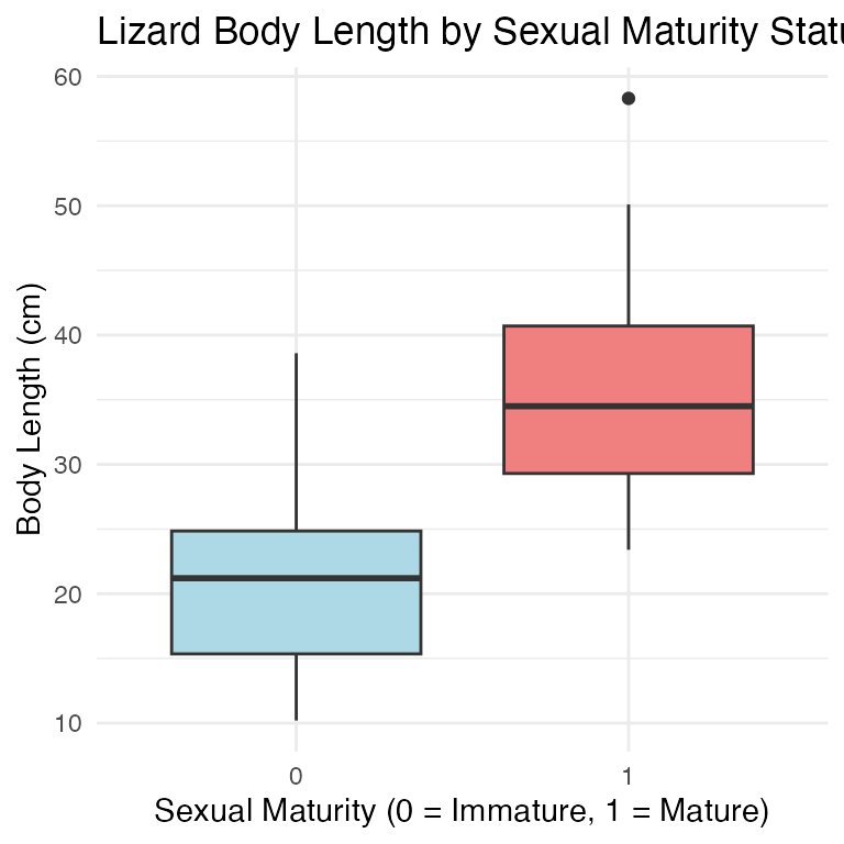
Let’s visualize how body length differs between sexually mature and immature lizards:

# Create boxplot showing length by maturity status
maturity_boxplot <- ggplot(lizards_df, aes(x = factor(mature), y = length)) +
  geom_boxplot(fill = c("lightblue", "lightcoral")) +
  labs(title = "Lizard Body Length by Sexual Maturity Status",
       x = "Sexual Maturity (0 = Immature, 1 = Mature)",
       y = "Body Length (cm)") +
  theme_minimal()

maturity_boxplot

What do we see?

• There appears to be a relationship between size and sexual maturity
• Mature lizards tend to be longer than immature ones
• But there’s overlap - not a perfect separation
• This suggests logistic regression might be appropriate

Step 3: Fit the Logistic Regression Model

Using glm() for Logistic Regression

The glm() function is similar to lm() but requires specifying the distribution family:

# Fit logistic regression model
# family = binomial tells R we have binary data
logistic_model <- glm(mature ~ length, 
                      data = lizards_df, 
                      family = binomial)

# Get model summary
summary(logistic_model)
## 
## Call:
## glm(formula = mature ~ length, family = binomial, data = lizards_df)
## 
## Coefficients:
##             Estimate Std. Error z value Pr(>|z|)   
## (Intercept)  -6.6899     2.1401  -3.126  0.00177 **
## length        0.2503     0.0775   3.229  0.00124 **
## ---
## Signif. codes:  0 '***' 0.001 '**' 0.01 '*' 0.05 '.' 0.1 ' ' 1
## 
## (Dispersion parameter for binomial family taken to be 1)
## 
##     Null deviance: 60.176  on 43  degrees of freedom
## Residual deviance: 34.041  on 42  degrees of freedom
## AIC: 38.041
## 
## Number of Fisher Scoring iterations: 6

Interpreting the Model Output

Coefficients:

• Intercept (β₀): -5.5847 - The log-odds when length = 0
• Slope (β₁): 0.2503 - Change in log-odds for each 1 cm increase in length

P-values:

• Both coefficients are significant (p < 0.05)
• We reject the null hypothesis that β₁ = 0
• There IS a relationship between length and sexual maturity

Understanding the Slope:

The positive slope (0.2503) indicates: - Longer lizards are more likely to be sexually mature - For each 1 cm increase in length, the log-odds of maturity increase by 0.2503

Step 4: Convert Log-Odds to Odds

Making the Results More Interpretable

Log-odds are hard to interpret. Let’s convert to odds:

# Extract the slope coefficient
slope_coefficient <- coef(logistic_model)[2]

# Convert log-odds to odds ratio
odds_ratio <- exp(slope_coefficient)
odds_ratio
##   length 
## 1.284388

# Interpretation
# For every 1 cm increase in length, the odds of being sexually mature
# increase by a factor of 1.284 (or about 28.4%)

Step 5: Create the Logistic Regression Plot

Visualizing the Probability Curve

# Create sequence of x-values for prediction
xvals <- seq(from = 10, to = 50, by = 0.01)

# Get predicted probabilities
yvals <- predict(logistic_model, 
                 list(length = xvals), 
                 type = "response")

# Create prediction dataframe for plotting
prediction_df <- data.frame(length = xvals, 
                           probability = yvals)

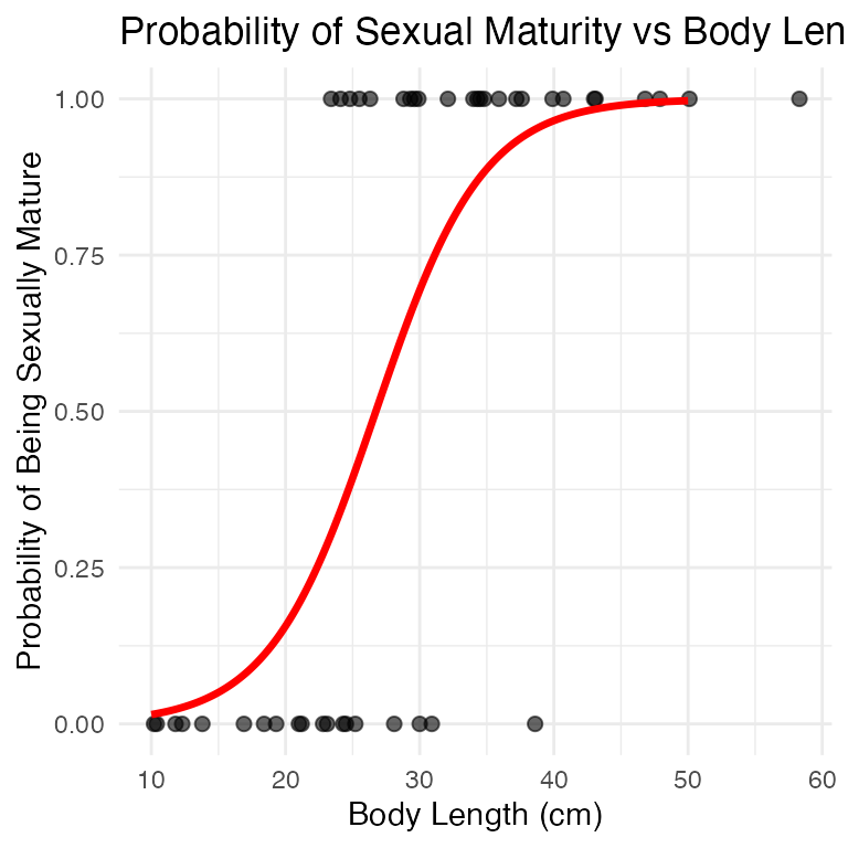
# Create the logistic regression plot
logistic_plot <- ggplot() +
  # Add data points
  geom_point(data = lizards_df, 
             aes(x = length, y = mature),
             alpha = 0.6, size = 2) +
  # Add logistic curve
  geom_line(data = prediction_df,
            aes(x = length, y = probability),
            color = "red", size = 1.2) +
  labs(title = "Probability of Sexual Maturity vs Body Length",
       x = "Body Length (cm)",
       y = "Probability of Being Sexually Mature") +
  theme_minimal()

logistic_plot

What the S-curve tells us:

• The red line shows how probability changes with length
• Small lizards (<20 cm) have very low probability of being mature
• Large lizards (>40 cm) have very high probability of being mature
• The steepest change occurs around 25-30 cm

Step 6: Making Predictions

Using the Model for Prediction

Let’s predict the probability of sexual maturity for specific lizard sizes:

# Predict for a 20 cm lizard
prob_20cm <- predict(logistic_model, 
                     list(length = 20), 
                     type = "response")
prob_20cm
##         1 
## 0.1565304

# Predict for a 30 cm lizard
prob_30cm <- predict(logistic_model, 
                     list(length = 30), 
                     type = "response")
prob_30cm
##         1 
## 0.6939292

# Predict for a 40 cm lizard
prob_40cm <- predict(logistic_model, 
                     list(length = 40), 
                     type = "response")
prob_40cm
##         1 
## 0.9651551

Interpretation:

• A 20 cm lizard has about 14% probability of being sexually mature
• A 30 cm lizard has about 70% probability of being sexually mature
• A 40 cm lizard has about 96% probability of being sexually mature

Step 7: Model Fit Assessment

Calculating Pseudo-R2 Values

Unlike linear regression, logistic regression doesn’t have a traditional R². We use pseudo-R² instead:

# Calculate pseudo-R2 values using pscl package
pseudo_r2 <- pR2(logistic_model)
## fitting null model for pseudo-r2
pseudo_r2
##         llh     llhNull          G2    McFadden        r2ML        r2CU 
## -17.0204762 -30.0881077  26.1352630   0.4343122   0.4478763   0.6009400

Interpreting Pseudo-R2 Values

The last three values are the pseudo-R² statistics:

• McFadden: Compares model to null model
• r2ML: Maximum likelihood based R²
• r2CU: Cragg-Uhler (Nagelkerke) R²

Values around 0.4-0.5 indicate moderate to good fit. Our model explains approximately 40-50% of the variation in sexual maturity status.

Step 8: Additional Diagnostics

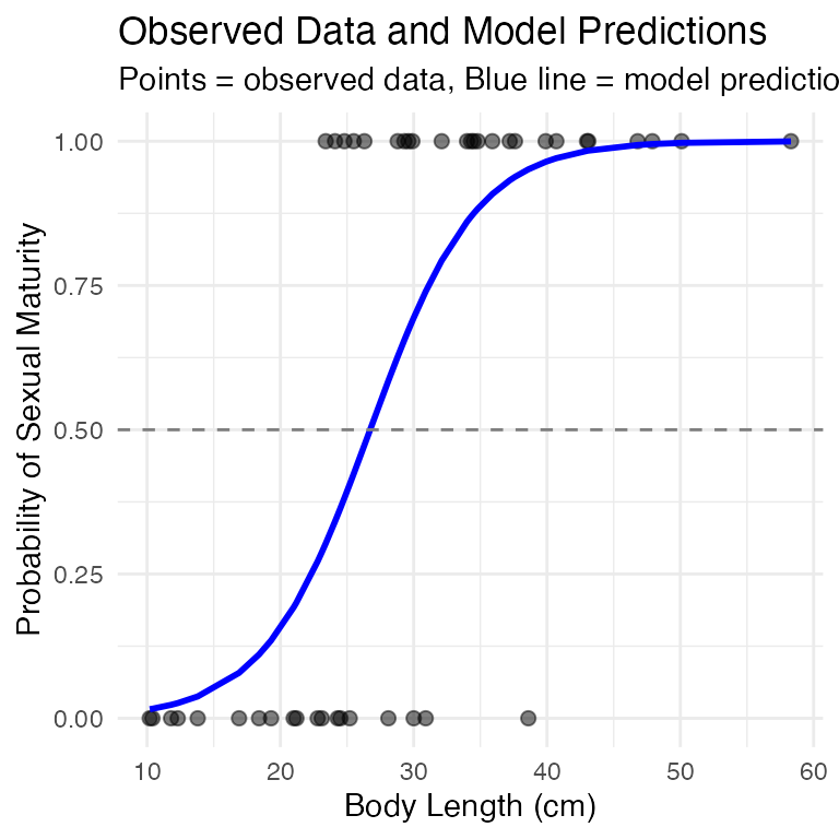
Creating a More Detailed Summary Plot

# Create a plot showing observed vs predicted probabilities
lizards_df$predicted_prob <- predict(logistic_model, type = "response")

diagnostic_plot <- ggplot(lizards_df, aes(x = length)) +
  # Add observed data as points
  geom_point(aes(y = mature), alpha = 0.5, size = 2) +
  # Add predicted probabilities
  geom_line(aes(y = predicted_prob), color = "blue", size = 1) +
  # Add 50% probability threshold
  geom_hline(yintercept = 0.5, linetype = "dashed", color = "gray50") +
  labs(title = "Observed Data and Model Predictions",
       x = "Body Length (cm)",
       y = "Probability of Sexual Maturity",
       subtitle = "Points = observed data, Blue line = model predictions") +
  theme_minimal()

diagnostic_plot

Summary: Key Takeaways

What We Learned:

1. Logistic regression models probability of binary outcomes
2. Uses glm() with family = binomial
3. Coefficients represent changes in log-odds
4. Convert to odds ratios for interpretation: exp(coefficient)
5. Creates S-shaped probability curves
6. Use pseudo-R² to assess model fit

Our Results:

• Significant positive relationship between body length and sexual maturity
• Each 1 cm increase in length increases odds of maturity by ~28%
• Model explains ~40-50% of variation in maturity status
• Can predict probability of maturity for any given length

When to Use Logistic Regression:

• Binary response variable (0/1, yes/no, success/failure)
• Want to predict probabilities
• Relationships that follow S-shaped curves
• When assumptions of linear regression are violated