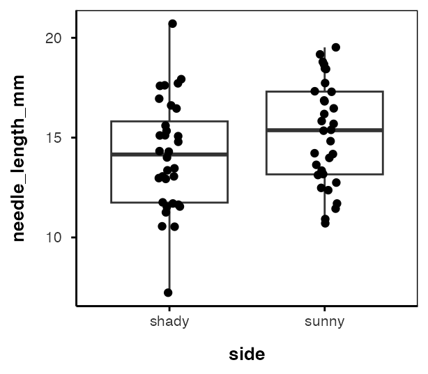
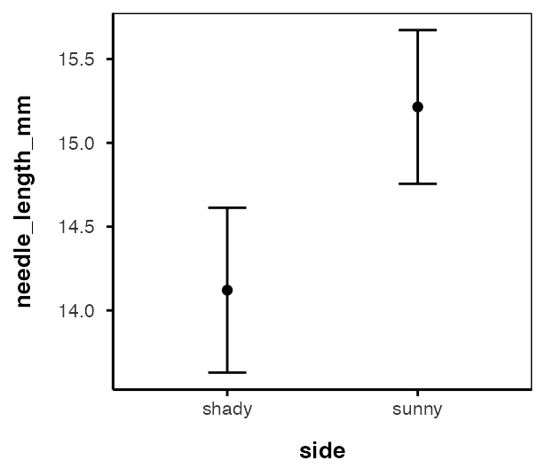
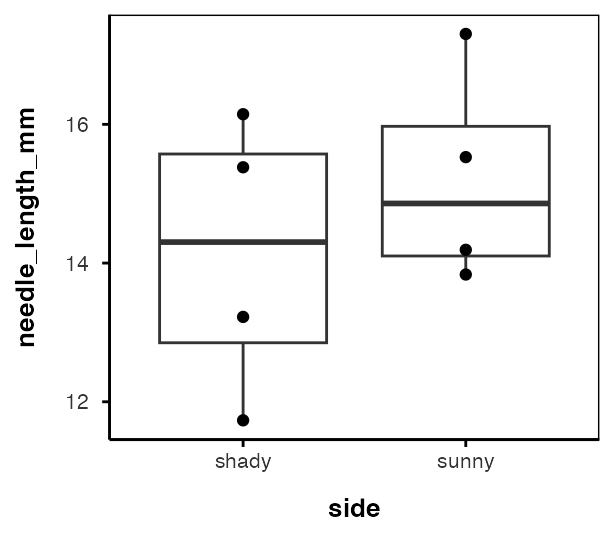
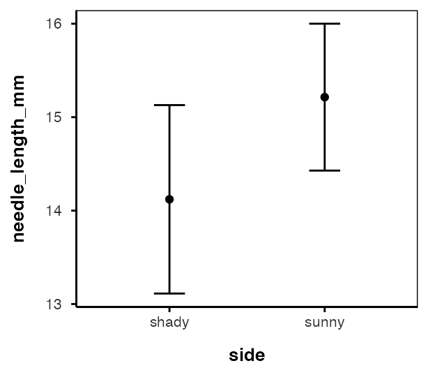
Lecture: T-Tests: One, Two, Paired

Comparing means

Bill Perry

Where We Left Off

Last time:

  • Histograms / frequency distributions
  • Probability distribution functions (PDFs)
  • Z-scores and t-scores
  • Tests of means using t-tests: one sample, two sample

Note

✅ Key idea from last lecture

A t-score is just a z-score computed with the sample standard deviation instead of the population standard deviation — that substitution is why we need the t-distribution at all. Today we put it to work.
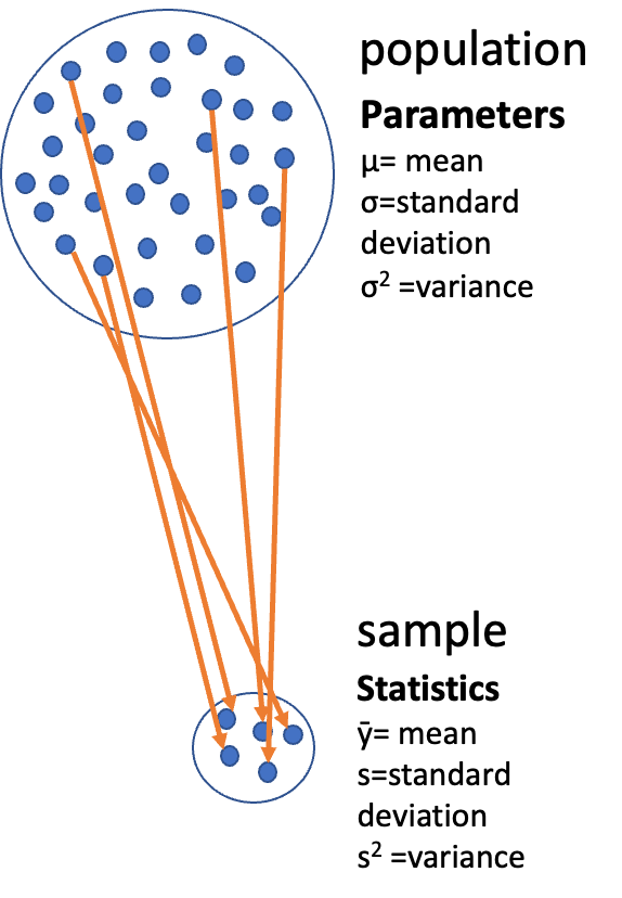
Diagram of a large circle labeled ‘population’ with dots representing individuals and Greek-letter parameters (mu, sigma, sigma-squared), with orange arrows showing a subset of dots being drawn down into a small circle labeled ‘sample’ with its statistics (y-bar, s, s-squared), illustrating that a sample is used to estimate unknown population parameters.

Note

Today’s roadmap

  1. Hypothesis testing framework
  2. The t-distribution
  3. One-sample t-test
  4. Two-sample t-test (Student’s and Welch’s)
  5. Paired t-test
  6. Checking assumptions throughout

Part 1 · Our Data

Setup — Loading the Class Pine Needle Data

library(readxl)
library(tidyverse)
library(patchwork)
library(car)   # For diagnostic tests

pine_df        <- read_excel("data/class_pine needle length.xlsx")
pine_switch_df <- read_excel("data/class_pine needle length switched.xlsx")

glimpse(pine_df)
Rows: 361
Columns: 5
$ group     <chr> "five", "five", "five", "five", "five", "five", "five", "fiv…
$ tree_no   <dbl> 1, 1, 1, 1, 1, 1, 1, 1, 1, 1, 1, 1, 1, 1, 1, 1, 1, 1, 1, 1, …
$ tree_char <chr> "tree_1", "tree_1", "tree_1", "tree_1", "tree_1", "tree_1", …
$ side      <chr> "sunny", "sunny", "sunny", "sunny", "sunny", "sunny", "sunny…
$ length_mm <dbl> 22.66, 21.14, 18.55, 18.65, 20.99, 18.94, 19.75, 18.46, 20.5…

Note

✅ Key idea

For two sample T-tests, degrees of freedom = n₁ + n₂ − 2. Once we average the needles up to one value per tree side (next slide), we have 8 trees per side — so df = 8 + 8 − 2 = 14. Note that n is the number of trees, not needles.

Tip

🖐 Recap

group is the class team, tree_no/tree_char identify the tree, side is sunny vs. shady, length_mm is the needle length.

Averaging Out Pseudoreplication

# Multiple needles per tree side are pseudoreplicates —
# average them so each tree/side is ONE data point
p_df <- pine_df %>%
  group_by(group, tree_no, tree_char, side) %>%
  summarise(length_mm = mean(length_mm, na.rm = TRUE), .groups = "drop")

ps_df <- pine_switch_df %>%
  group_by(group, tree_no, tree_char, side) %>%
  summarise(length_mm = mean(length_mm, na.rm = TRUE), .groups = "drop")

ps_shady_df <- ps_df %>% filter(side == "shady")
ps_sunny_df <- ps_df %>% filter(side == "sunny")

Important

Why average first? The true experimental unit here is tree side, not needle. Treating every needle as independent would inflate our sample size and our confidence — the same pseudoreplication trap from earlier in the course.

stats_df <- ps_df %>%
  group_by(side) %>%
  summarize(
    mean_length = mean(length_mm, na.rm = TRUE),
    sd_length   = sd(length_mm, na.rm = TRUE),
    se_length   = sd(length_mm, na.rm = TRUE) / sum(!is.na(length_mm))^.5,
    count       = sum(!is.na(length_mm)),
    .groups = "drop"
  )
stats_df
# A tibble: 2 × 5
  side  mean_length sd_length se_length count
  <chr>       <dbl>     <dbl>     <dbl> <int>
1 shady        17.6      2.51     0.886     8
2 sunny        16.2      2.64     0.934     8

The Data — Two Versions

p_plot <- p_df %>%
  ggplot(aes(side, length_mm, fill = side)) +
  geom_boxplot(alpha = 0.7) +
  geom_point(aes(group = group, color = group)) +
  geom_line(aes(group = group, color = group)) +
  labs(x = "Side of tree", y = "Length (mm)", caption = "Pine needles") +
  theme_minimal(base_size = 9) +
  theme(legend.position = "none")
p_plot

Boxplot of needle length by side of tree (shady vs. sunny) from the original (unswitched) pine needle file, with points for each field team connected by a line, showing each team's shady and sunny values.

Warning

⚠️ Watch out!

class_pine needle length switched.xlsx has the sunny/shady labels swapped relative to the original file. From here on, ps_df (the switched version) is the dataset we’ll actually test — it’s the one that matches the field notes.

The Data We’ll Test — ps_df

ps_plot <- ps_df %>%
  ggplot(aes(side, length_mm, fill = side)) +
  geom_boxplot(alpha = 0.7) +
  geom_point(aes(group = group, color = group)) +
  geom_line(aes(group = group, color = group)) +
  labs(x = "Side of tree", y = "Length (mm)", caption = "Pine needles switched") +
  theme_minimal(base_size = 9) +
  theme(legend.position = "none")
ps_plot

Boxplot of needle length by side of tree (shady vs. sunny) from the corrected, switched-labels pine needle file, with points for each field team connected by a line — this is the dataset used for the rest of the analysis.

Goals for today, using ps_df:

  • Statistical inference fundamentals
  • Hypothesis testing principles
  • t-distributions
  • One-sample, two-sample, and paired t-tests
  • Assumption tests

Part 2 · Hypothesis Testing Framework

Hypothesis Testing — the Key Components

Hypothesis testing is a systematic way to evaluate research questions using data.

Key components:

  1. Null hypothesis (H₀) — typically “no effect” or “no difference”
  2. Alternative hypothesis (Hₐ) — the claim we’re trying to support
  3. Statistical test — method for evaluating evidence against H₀
  4. P-value — probability of observing our result (or more extreme) if H₀ is true
  5. Significance level (α) — threshold for rejecting H₀, typically 0.05

Decision rule: Reject H₀ if p-value < α.

Note

📖 Reference

Gotelli & Ellison, A Primer of Ecological Statistics, Ch. 4 — Framing and Testing Hypotheses (Statistical Significance and P-Values).

The Logic of a Statistical Test

A test assesses the likelihood of the null hypothesis being true.

  • If H₀ is likely false, Hₐ is assumed correct
  • More precisely: the long-run probability of obtaining our sample value (or a more extreme one) if the null hypothesis is true
  • Written p(data | H₀) — the probability of the data, given H₀

Note

✅ Key idea

p(data | H₀) is not the same as p(H₀ | data). A t-test never tells you the probability that H₀ is true — only how surprising your data would be if it were.

p-value range Interpretation
p > 0.10 No evidence against H₀
0.05 < p < 0.10 Weak evidence against H₀
0.01 < p < 0.05 Moderate evidence against H₀
0.001 < p < 0.01 Strong evidence against H₀
p < 0.001 Very strong evidence against H₀

Part 3 · The t-Distribution

One-Tailed Questions

One-tailed questions ask about the area of the distribution to the left (or right) of a certain value, for a one-sample test.

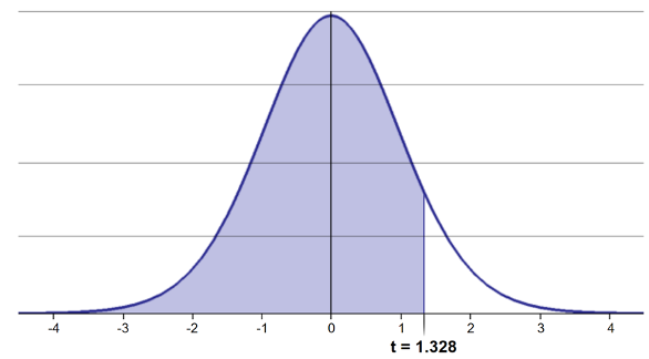
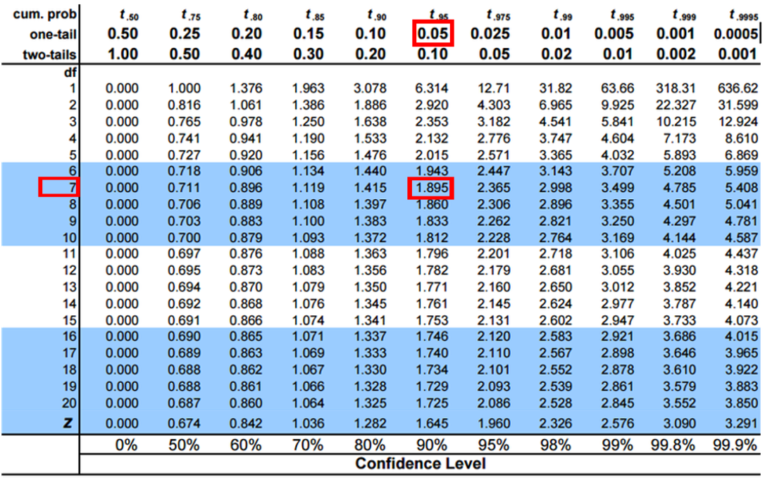
  • n = 8 (df = 7) — 95% of the observations found to the left
  • t = 1.895 (5% are outside)

Bell-shaped t-distribution curve with the area to the left of the critical value shaded, illustrating a one-tailed cutoff where the shaded region represents the proportion of the distribution below that t-value (here t = 1.895 at df = 7).

Student’s t critical-value table with the one-tail 0.05 column and df = 7 row highlighted, intersecting at the critical value 1.895, the value used for a one-tailed test at alpha = 0.05.

Two-Tailed Questions

Two-tailed questions refer to the area between certain values.

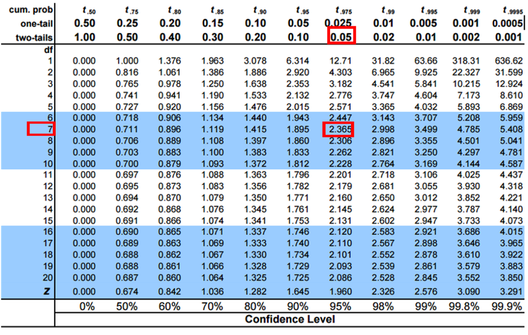
  • n = 8 (df = 7), 95% of the observations are between t = −2.365 and t = 2.365 (2.5% outside on each side)
  • Compare to the one-tailed cutoff: t = 1.895 (5% outside)
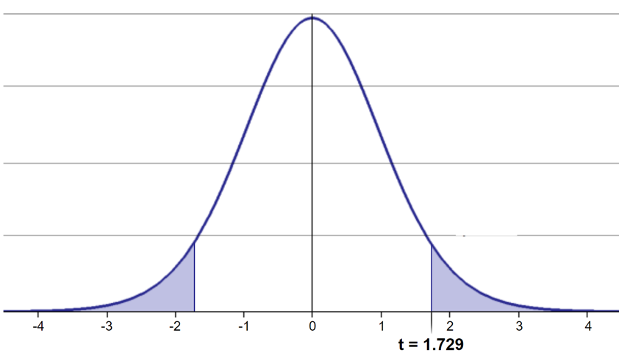
Bell-shaped t-distribution curve with both tails shaded beyond the critical values (here t = -2.365 and t = 2.365 at df = 7), illustrating a two-tailed cutoff where the two shaded regions together represent the proportion of the distribution outside that range.

Student’s t critical-value table with the two-tail 0.05 column and df = 7 row highlighted, intersecting at the critical value 2.365, the value used for a two-tailed test/95% confidence interval at alpha = 0.05.

Tip

🖐 Notice

The two-tailed critical value is farther from zero than the one-tailed value — splitting 5% into two tails means each tail only gets 2.5%.

Calculating a Confidence Interval

Using a two-sided test:

\[\text{CI} = \bar{y} \pm t \cdot \frac{s}{\sqrt{n}}\]

  • 95% CI, Sample A: 17.6 ± 2.365 × (2.51 / 8^0.5) = ± 2.10
  • The 95% CI is between 15.50 and 19.70
  • “The 95% CI for the population mean from sample A is 17.6 ± 2.1”

Note

📖 Reference

Whitlock & Schluter, Analysis of Biological Data, Ch. 11 — Inference for a Normal Population.

Student’s t critical-value table with the two-tail 0.05 column and df = 7 row highlighted, intersecting at the critical value 2.365, the value used for a two-tailed test/95% confidence interval at alpha = 0.05.

Applications of the t-Distribution

  • Can assess confidence that the population mean is within a certain range
  • Can use the t-distribution to ask:
    • “What is the probability of getting a sample with mean = ȳ from a population with mean = µ?” (1-sample t-test)
    • “What is the probability that two samples came from the same population?” (2-sample t-test)

Tip

🖐 Try it yourself

Before the next slide: which of these two questions do you think a one-sample t-test answers, and which needs a two-sample t-test?

Part 4 · One-Sample T-Test

One-Sample T-Test — Hypotheses and Assumptions

We want to test if the mean needle length on the shady side differs from 15mm.

Activity: define hypotheses and identify assumptions

  • H₀: μ = 15 (the mean needle length on the shady side is 15mm)
  • Hₐ: μ ≠ 15 (the mean needle length on the shady side is not 15mm)

Assumptions for a t-test:

  1. Data is normally distributed
  2. Observations are independent
  3. No significant outliers

Note

📖 Reference

Whitlock & Schluter, Ch. 11, covers the one-sample t-test as the simplest hypothesis test on a normally distributed variable.

Checking Normality — QQ Plot

# The one-sample test below is on the SHADY side, so that is the group
# whose normality we need to check -- not the two sides pooled together.
qqPlot(ps_shady_df$length_mm,
       main = "QQ Plot — shady side needle length",
       ylab = "Sample Quantiles")

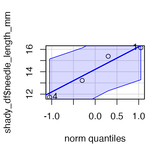
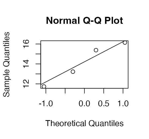
QQ-plot of pine needle length with a confidence envelope, used to visually check whether needle length is approximately normally distributed.

[1] 7 6

Tip

🖐 Notice

Points that hug the blue line support normality; points that curve away — especially in the tails — are a warning sign.

Checking Normality — Shapiro-Wilk Test

shapiro.test(ps_shady_df$length_mm)

    Shapiro-Wilk normality test

data:  ps_shady_df$length_mm
W = 0.96639, p-value = 0.8683

Important

H₀ for Shapiro-Wilk is “the data ARE normal.” A non-significant result (p > 0.05) is what we’re hoping for here — it means we fail to reject normality.

Tip

🖐 Why the shady side only?

We test the group the hypothesis is about. Pooling shady and sunny would mix two distributions with different means, which can look non-normal even when each group is perfectly normal.

Checking for Outliers

shady_sunny_plot <- ps_df %>%
  ggplot(aes(x = side, y = length_mm, fill = side)) +
  geom_boxplot() +
  labs(x = "side", y = "Length (mm)", fill = "side") +
  theme_minimal(base_size = 9)
shady_sunny_plot

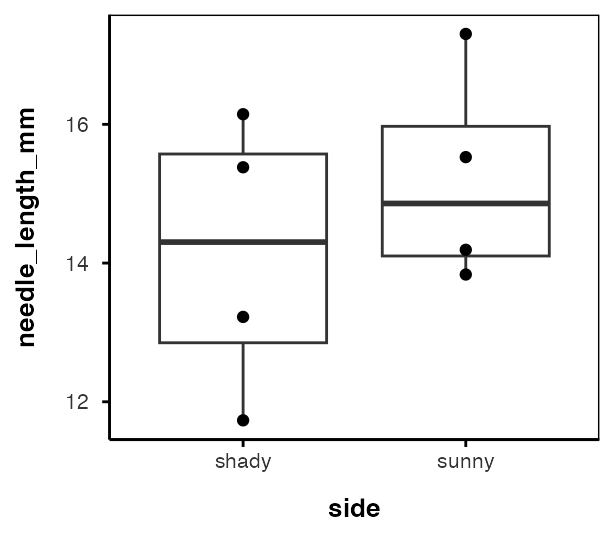
Boxplot of pine needle length by side of tree (shady vs. sunny), used to visually check for outliers before running t-tests.

Tip

Points beyond the whiskers are potential outliers — always look before you test.

Practice Exercise 1: One-Sample t-Test

Tip

Practice Exercise 1: One-sample t-test

Let’s perform a one-sample t-test to determine if the mean needle length on the shady side differs from 15mm:

ps_shade_mean <- mean(ps_shady_df$length_mm, na.rm = TRUE)
cat("Mean:", round(ps_shade_mean, 1), "mm\n")
Mean: 17.6 mm
t_test_result <- t.test(ps_shady_df$length_mm, mu = 15)
t_test_result

    One Sample t-test

data:  ps_shady_df$length_mm
t = 2.9414, df = 7, p-value = 0.02167
alternative hypothesis: true mean is not equal to 15
95 percent confidence interval:
 15.51092 19.70030
sample estimates:
mean of x 
 17.60561 

Interpret this test result by answering these questions:

  1. What was the null hypothesis?
  2. What was the alternative hypothesis?
  3. What does the p-value tell us?
  4. Should we reject or fail to reject the null hypothesis at α = 0.05?
  5. What is the practical interpretation of this result for botanists?

Visualizing the One-Sample Test — t Scale
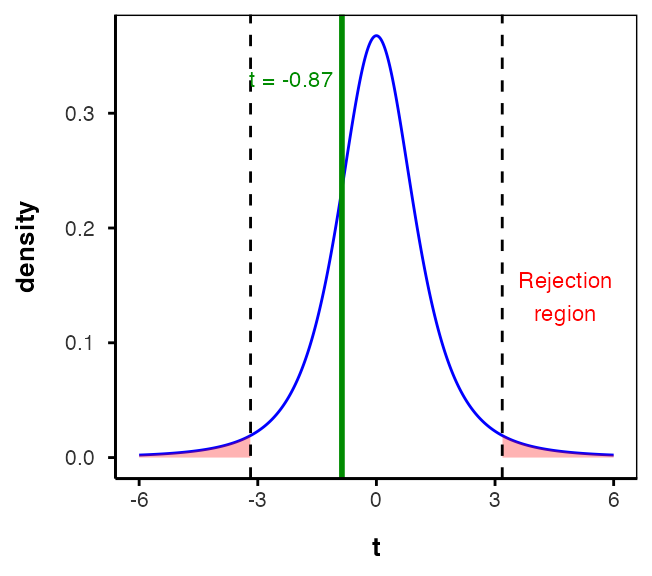
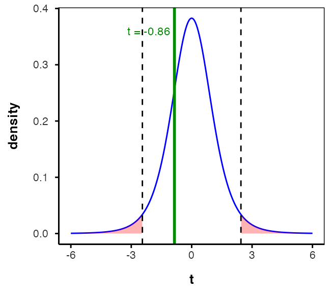
T-distribution curve for the one-sample test, with the two-tailed rejection region shaded red, a dashed line at the critical t-value, and a solid green line marking the observed t-statistic, which falls inside the rejection region.

Note

✅ Key idea

The green line (our observed t) falls inside the red rejection region — that’s what “significant” looks like on a t-distribution.

Visualizing the One-Sample Test — Original Units
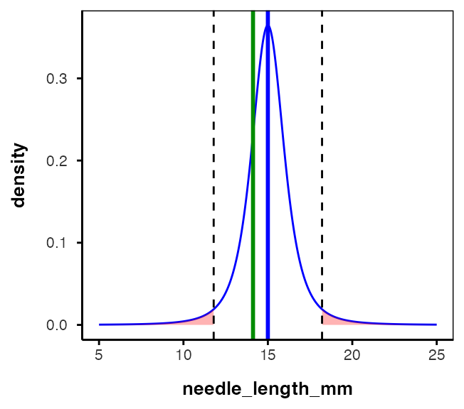
The same one-sample t-test rejection region re-plotted on the original millimeter measurement scale instead of the t-statistic scale, with vertical lines marking the hypothesized mean (15mm, blue) and observed sample mean (green).

Tip

🖐 Notice

Same test, same conclusion — just relabeled onto the millimeter scale instead of the t scale. The blue line (H₀ = 15) sits outside the sample’s plausible range.

Interpreting the One-Sample T-Test

Activity: interpret the t-test results

  • What does the p-value tell us?
  • Should we reject or fail to reject the null hypothesis?

Note

How to report this result in a scientific paper

“A one-sample t-test at α = 0.05 showed that the mean needle length (… mm, SD = …) [was/was not] significantly different from the expected 15mm, t(…) = …, p = …”

Part 5 · Two-Sample T-Test

Two-Sample T-Tests — Introduction

For example — what is the probability that population X is the same as population Y?

How would you assess this question using what we learned?

This is what we will do with the needle length again…

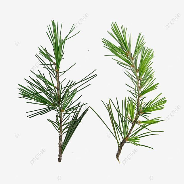
Photo of two separate green pine branches side by side, each with needle clusters, representing the two independent samples (populations X and Y) being compared in a two-sample t-test.

Comparing Two Samples

What is the probability that population X is the same as population Y?

How would you assess this question using what we learned?

shady_sunny_plot

The boxplot of pine needle length by side of tree, repeated here as a lead-in to the two-sample t-test comparing the two sides.

Tip

🖐 Try it yourself

Based on the boxplot alone, what would you guess the two-sample t-test will conclude about needle length on the two sides?

Practice Exercise 2: Formulating Hypotheses

Tip

Practice Exercise 2: Formulating hypotheses

For the following research question about needle lengths, write the null and alternative hypotheses:

Are needle lengths on shady and sunny sides different?

H0 =
Ha =

Two-Sample T-Test Framework

Now let’s compare needle lengths from the two sides.

Question: Is there a significant difference in needle length between the sides?

This requires a two-sample t-test, which compares means from two independent groups.
\[t = \frac{\bar{x}_1 - \bar{x}_2}{S_p\sqrt{\frac{1}{n_1} + \frac{1}{n_2}}}\]

Where:

  • x̄₁, x̄₂: sample means of the two groups
  • s²ₚ: pooled variance = [(n₁−1)s₁² + (n₂−1)s₂²] / (n₁+n₂−2)
  • Sₚ = √s²ₚ: the pooled standard deviation (that’s what appears in the formula)
  • n₁, n₂: sample sizes of the two groups
  • Sₚ√(1/n₁ + 1/n₂): the standard error of the difference — the whole denominator, not just the square-root term

\[t = \frac{\text{SIGNAL}}{\text{NOISE}}\]

Note

📖 Reference

Whitlock & Schluter, Ch. 12 — Comparing Two Means.

Practice Exercise 3: Summary Statistics

Tip

Practice Exercise 3: Calculate summary statistics grouped by side

Before conducting the test, we need to understand the data for each group.

group_summary <- ps_df %>%
  group_by(side) %>%
  summarize(
    mean_length = mean(length_mm, na.rm = TRUE),
    sd_length   = sd(length_mm, na.rm = TRUE),
    n           = sum(!is.na(length_mm)),
    se_length   = sd_length / sqrt(n),
    .groups = "drop"
  )
group_summary
# A tibble: 2 × 5
  side  mean_length sd_length     n se_length
  <chr>       <dbl>     <dbl> <int>     <dbl>
1 shady        17.6      2.51     8     0.886
2 sunny        16.2      2.64     8     0.934

Practice Exercise 4: Effect Size

Tip

Practice Exercise 4: Effect size

We could also look at the difference in means:

group_summary %>%
  summarize(difference = mean_length[side == "shady"] - mean_length[side == "sunny"])
# A tibble: 1 × 1
  difference
       <dbl>
1       1.45

Practice Exercise 5: Plotting Mean ± SE Directly

Tip

Practice Exercise 5: Using ggplot to get a summary plot

ggplot can compute and plot the mean and standard error directly:

needle_mean_se_plot <- ggplot(ps_df, aes(x = side, y = length_mm, color = side)) +
  stat_summary(fun = mean, geom = "point") +
  stat_summary(fun.data = mean_se, geom = "errorbar", width = 0.2) +
  labs(x = "side", y = "Mean Length (mm)") +
  theme_classic(base_size = 9)
needle_mean_se_plot

Point-and-error-bar plot of mean needle length ± standard error for the shady and sunny sides.

Testing Assumptions for a Two-Sample T-Test

For a two-sample t-test, we need to check:

  1. Normality within each group
  2. Equal variances between groups (for the standard t-test)
  3. Independent observations

If assumptions are violated:

  • Welch’s t-test (unequal variances)
  • Non-parametric alternatives (Mann-Whitney U test)

Note

📖 Reference

Whitlock & Schluter, Ch. 13 — Handling Violations of Assumptions, covers non-parametric alternatives when normality or equal variance fails.

Practice Exercise 6: Separate Group Data

Tip

Practice Exercise 6: separate group data

Note you need to test each group separately for normality — first, split the data:

head(ps_shady_df)
# A tibble: 6 × 5
  group                      tree_no tree_char side  length_mm
  <chr>                        <dbl> <chr>     <chr>     <dbl>
1 big_fat_fecund_female_fish       2 tree_2    shady      15.4
2 bill                             3 tree_3    shady      16.7
3 ciabatta                         5 tree_5    shady      19.1
4 fake_data                        8 tree_8    shady      17.4
5 five                             1 tree_1    shady      20.3
6 moose_walkin                     7 tree_7    shady      20.7
head(ps_sunny_df)
# A tibble: 6 × 5
  group                      tree_no tree_char side  length_mm
  <chr>                        <dbl> <chr>     <chr>     <dbl>
1 big_fat_fecund_female_fish       2 tree_2    sunny      13.2
2 bill                             3 tree_3    sunny      16.0
3 ciabatta                         5 tree_5    sunny      17.7
4 fake_data                        8 tree_8    sunny      13.0
5 five                             1 tree_1    sunny      19.9
6 moose_walkin                     7 tree_7    sunny      18.4

Practice Exercise 7: Combined Normality Test

Tip

Practice Exercise 7: test normality at one time

There are always a lot of ways to do this in R:

normality_results <- ps_df %>%
  group_by(side) %>%
  summarize(
    shapiro_stat    = shapiro.test(length_mm)$statistic,
    shapiro_p_value = shapiro.test(length_mm)$p.value,
    normal_distribution = if_else(shapiro_p_value > 0.05, "Normal", "Non-normal"))
normality_results
# A tibble: 2 × 4
  side  shapiro_stat shapiro_p_value normal_distribution
  <chr>        <dbl>           <dbl> <chr>              
1 shady        0.966           0.868 Normal             
2 sunny        0.900           0.289 Normal             

Practice Exercise 8: Test Equal Variances

Tip

Practice Exercise 8: test equal variances

Levene’s test can be done on the original data frame.

Note: the Levene’s test result should be NOT significant — what is the null hypothesis here?

# leveneTest needs the grouping variable as a factor
levene_result <- leveneTest(length_mm ~ factor(side), data = ps_df)
print("Levene's Test for Homogeneity of Variance:")
[1] "Levene's Test for Homogeneity of Variance:"
print(levene_result)
Levene's Test for Homogeneity of Variance (center = median)
      Df F value Pr(>F)
group  1  0.2062 0.6567
      14               

Conducting the Two-Sample T-Test — Standard

Now we can compare the mean needle lengths between shady and sunny sides.

  • H₀: μ₁ = μ₂ (the needle lengths do not differ)
  • Hₐ: μ₁ ≠ μ₂ (the mean needle lengths differ — direction not specified)

Deciding between:

  • Standard t-test (equal variances)
  • Welch’s t-test (unequal variances)
# Use var.equal = TRUE for standard t-test,
# var.equal = FALSE for Welch's t-test
t_test_result <- t.test(length_mm ~ side, data = ps_df, var.equal = TRUE)
print("Standard two-sample t-test:")
[1] "Standard two-sample t-test:"
print(t_test_result)

    Two Sample t-test

data:  length_mm by side
t = 1.1279, df = 14, p-value = 0.2783
alternative hypothesis: true difference in means between group shady and group sunny is not equal to 0
95 percent confidence interval:
 -1.309330  4.214005
sample estimates:
mean in group shady mean in group sunny 
           17.60561            16.15328 

Conducting the Two-Sample T-Test — Welch’s

Now we can compare the mean needle lengths between shady and sunny sides.

  • H₀: μ₁ = μ₂ (the needle lengths do not differ)
  • Hₐ: μ₁ ≠ μ₂ (the mean needle lengths differ — direction not specified)

Deciding between:

  • Standard t-test (equal variances)
  • Welch’s t-test (unequal variances)
t_test_result <- t.test(length_mm ~ side, data = ps_df, var.equal = FALSE)
print("Welch's two-sample t-test:")
[1] "Welch's two-sample t-test:"
print(t_test_result)

    Welch Two Sample t-test

data:  length_mm by side
t = 1.1279, df = 13.96, p-value = 0.2784
alternative hypothesis: true difference in means between group shady and group sunny is not equal to 0
95 percent confidence interval:
 -1.310069  4.214743
sample estimates:
mean in group shady mean in group sunny 
           17.60561            16.15328 

Standard vs. Welch’s t-Test

Standard t-test (Student’s t-test)

  • Assumes equal variances between groups
  • Uses a pooled variance estimate combining both groups
  • Has higher statistical power when the equal-variance assumption is met
  • Degrees of freedom = n₁ + n₂ − 2

Welch’s t-test

  • Does not assume equal variances (the “unequal variances t-test”)
  • Uses separate variance estimates for each group
  • More robust when group variances differ
  • Uses the Welch-Satterthwaite equation — df is typically non-integer and smaller than the standard t-test’s

Interpreting the Two-Sample T-Test

Interpret the results of the two-sample t-test

What can we conclude about needle lengths on the sunny vs. shady sides?

Note

How to report this result in a scientific paper

“A two-tailed, two-sample t-test at α = 0.05 showed [a significant/no significant] difference in needle length between sunny (M = …, SD = …) and shady (M = …, SD = …) sides of pine trees, t(…) = …, p = …”

T-distribution curve with 14 degrees of freedom for the two-sample needle-length test, red rejection regions in both tails beyond the critical t-values of plus and minus 2.145, and a dashed blue line marking the observed t-statistic of 1.128, which falls inside the light blue non-rejection region.

Part 6 · Paired T-Test

What Does a Paired T-Test Tell Us?

Paired t-test:

  • Compares two measurements from the same subjects or matched pairs
  • Tests whether the mean difference between paired observations equals zero
  • Examples: before/after measurements on the same individuals, left vs. right measurements, matched case-control studies
  • Uses the differences between pairs as the data
  • Generally more powerful, because it controls for individual variation

Note

📖 Reference

Whitlock & Schluter, Ch. 12, section on the paired design.

ps_wide_df <- ps_df %>%
  pivot_wider(
    names_from = "side",
    values_from = length_mm
  )

paired_t_test_result <- t.test(ps_wide_df$sunny, ps_wide_df$shady, paired = TRUE)
print("Paired t-test:")
[1] "Paired t-test:"
print(paired_t_test_result)

    Paired t-test

data:  ps_wide_df$sunny and ps_wide_df$shady
t = -2.7818, df = 7, p-value = 0.02723
alternative hypothesis: true mean difference is not equal to 0
95 percent confidence interval:
 -2.6868652 -0.2178092
sample estimates:
mean difference 
      -1.452337 

Same Data, Two Different Answers

Look carefully at what just happened — both tests used exactly the same 16 numbers:

Test t df p Conclusion
Two-sample 1.128 14 0.278 Not significant
Paired −2.782 7 0.027 Significant

Why the difference?

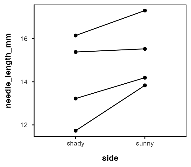
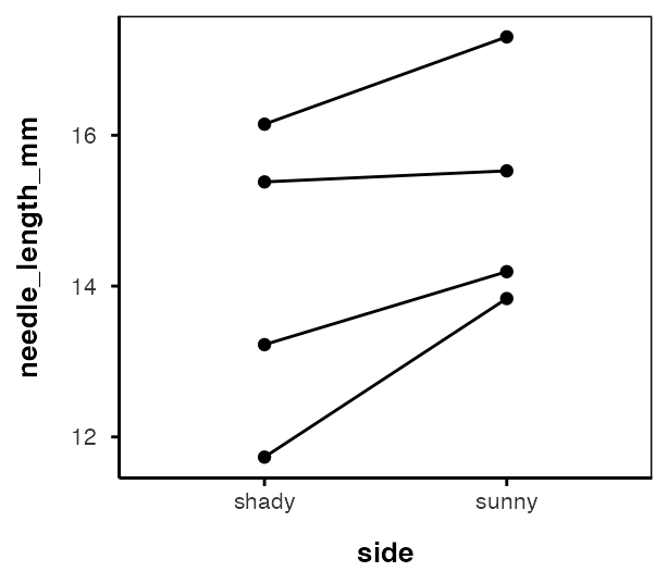
  • The two-sample test throws the pairing away. Tree-to-tree variation (some teams’ trees just have longer needles) lands in the noise, swamping the signal.
  • The paired test looks only at the shady−sunny difference within each tree, so tree-to-tree variation cancels out entirely.
Important

These data are paired by design — each team measured both sides of the same tree. The paired test is the correct one here; the two-sample test is the wrong tool, and it would have made us miss a real effect.

Slope plot showing each team's tree as a line connecting its shady value to its sunny value; nearly every line slopes downward from shady to sunny, showing a consistent within-tree effect even though the two groups overlap heavily overall.

What Is Going On?

Note that there is a lot of variation within trees, but the trend is the same across trees.

ps_plot

The needle length by side-of-tree boxplot with team lines, repeated to show within-tree variation alongside the consistent shady-vs-sunny trend across trees, motivating the paired t-test.

Part 7 · Assumptions and Wrap-Up

Assumptions of Parametric Tests

Common assumptions for t-tests:

  1. Normality — data comes from normally distributed populations
  2. Equal variances (for two-sample tests)
  3. Independence — observations are independent
  4. No outliers — extreme values can influence results

What can we do if our data violates these assumptions?

Alternatives when assumptions are violated:

  • Data transformation (log, square root, etc.)
  • Non-parametric tests
  • Robust statistical methods

Summary and Conclusions

In this lecture, we’ve:

  1. Formulated hypotheses about pine needle length
  2. Tested assumptions for parametric tests
  3. Conducted one-sample, two-sample, and paired t-tests
  4. Visualized data using appropriate methods
  5. Learned how to interpret and report t-test results

Note

Key takeaways

  • Always check assumptions before conducting tests
  • Visualize your data to understand patterns
  • Report results comprehensively
  • Consider alternatives when assumptions are violated — non-parametric tests, coming up soon