Lecture — One-Factor ANOVA: Start to Finish

Seven sites, one question: do these possums differ in size?

Bill Perry

2026-11-10

Where We Left Off — Two Groups

  • A t-test compared two group means
  • lm() fit a model and gave us slopes and intercepts
  • A factor let us decide what order groups sit in
  • And every time, we checked whether the test was allowed before we believed it

Note

✅ Transition

Today the question is the same shape — do these groups differ? — but there are seven groups, not two. That one change breaks the t-test, and the thing that replaces it is ANOVA. 🐾

Goals for Today

  • See why twenty-one t-tests is the wrong answer
  • Look at the data before testing anything
  • Use factor() to give groups names and an order
  • Fit with lm(), test with car::Anova(type = 2)
  • Check the assumptions after the fit:
    • performance::check_model()
    • car::leveneTest()
  • Say how big the effect is with eta-squared
  • Find out which groups differ — emmeans + letters
  • Write the result up in a sentence a reader can use

Tools today:

  • tidyverse
  • car — Anova(), leveneTest()
  • performance — check_model()
  • emmeans — follow-up tests
  • multcomp — the letters

Data: 🐾 104 brushtail possums, 7 sites, off Kaggle

Tip

Five chunks: why → look → test → check → which.

How to Use These Slides

Five short chunks. After each one you switch to the activity and run the code yourself.

Every line is already written for you. Your job is to run it, read the output, and argue with it.

Important

⚠️ Install first

install.packages("performance")
install.packages("see")
install.packages("emmeans")
install.packages("multcomp")

performance pulls in a dozen dependencies. Do it before class, not during.

Note

The homework is a separate file

19_anova_one_factor_homework.R — the same possums, measured a different way.

🧩 Chunk 1 of 5 · Why Not Just Do Lots of t-Tests?

We will cover: where the data came from, and the one arithmetic fact that kills the obvious approach.

The Animals

Mountain brushtail possum, Trichosurus cunninghami 🐾

  • A nocturnal, tree-dwelling Australian marsupial
  • 104 animals live-trapped at seven forest sites, from Victoria in the south up to Queensland
  • Each animal measured: head length, skull width, total length, tail length, plus age and sex

Our question today:

Do possums from different sites differ in total length?

Note

🧪 One factor, seven levels

  • Response: total_l, total length in cm — a number
  • Factor: site, which forest they were trapped in — seven groups

One factor. That is the whole design, and the name of the test.

The Obvious Idea — And Why It Fails

Seven groups. We know how to compare two. So: compare every pair?

Seven groups make 21 pairs. Twenty-one t-tests.

Each test at \(\alpha = 0.05\) has a 5% chance of a false positive. Run 21 of them on data where nothing is going on:

\[1 - 0.95^{21} = 0.66\]

A 66% chance of at least one “significant” result from pure noise.

Warning

⚠️ This is the whole problem

You would find something. You would find it two times out of three. And it would mean nothing.

More tests is not more rigour. More tests is more chances to fool yourself.

What ANOVA Does Instead

ANOVA asks one question first:

Is there any difference among these seven means?

One question, one p-value, one 5% risk.

It answers by comparing two kinds of variation:

  • Between groups — how far the site means sit from the overall mean
  • Within groups — how much possums at the same site differ from each other

\[F = \frac{\text{variation between groups}}{\text{variation within groups}}\]

Note

🧠 What F means

  • \(F \approx 1\) → groups differ about as much as individuals do. Nothing to see.
  • \(F \gg 1\) → groups differ more than individuals within them do. Something is going on.

“Analysis of variance” is a literal name.

🧩 Chunk 2 of 5 · Look at It First

We will cover: reading the file, turning site numbers into real names with factor(), and plotting before testing.

Read It In

# Load packages ---------------------------------------
library(tidyverse)
library(car)          # Anova(), leveneTest()
library(performance)  # check_model()
library(emmeans)      # follow-up comparisons
library(multcomp)     # the compact letter display

# Read the file ---------------------------------------
possum_raw <- read_csv("data/possum.csv")

dim(possum_raw)
[1] 104   8
names(possum_raw)
[1] "site"    "pop"     "sex"     "age"     "head_l"  "skull_w"
[7] "total_l" "tail_l" 
⚠️ One Side Effect of Loading multcomp

multcomp loads MASS, and MASS has its own select(). It masks the dplyr one.

So after today’s library() block, this quietly breaks:

possum_df %>% select(site, total_l)
#> Error: unused arguments

The fix is to say which one you mean:

possum_df %>% dplyr::select(site, total_l)

Warning

⚠️ Watch the startup messages

R told you this when you loaded the package. Nobody reads it.

select() is the usual casualty. filter() is the other one.

None of today’s code uses select() — but your code might.

The Site Column Is a Problem

possum_raw %>% count(site)
# A tibble: 7 × 2
   site     n
  <dbl> <int>
1     1    33
2     2    13
3     3     7
4     4     7
5     5    13
6     6    13
7     7    18

Warning

⚠️ Those are numbers, and R will treat them as numbers

site arrives as the integers 1–7. To R that is a quantity — as if site 6 were “twice site 3”. It is not. It is a name that happens to be written with a digit.

Leave it like this and lm() will fit a straight line through site number, which is nonsense.

Fix It With factor()

possum_df <- possum_raw %>%
  filter(!is.na(total_l)) %>%
  mutate(site_name = factor(site,
                            levels = 1:7,
                            labels = c("Cambarville", "Bellbird",
                                       "Whian Whian", "Byrangery",
                                       "Conondale", "Allyn River",
                                       "Bulburin")))

possum_df %>% count(site_name)
# A tibble: 7 × 2
  site_name       n
  <fct>       <int>
1 Cambarville    33
2 Bellbird       13
3 Whian Whian     7
4 Byrangery       7
5 Conondale      13
6 Allyn River    13
7 Bulburin       18

What Just Happened

factor(site,
       levels = 1:7,
       labels = c("Cambarville", ...))
  • levels = the values as they appear in the data
  • labels = what you want them called

The two lists must be the same length and in the same order. Get the order wrong and every single result is quietly mislabelled — no error, no warning.

The site names come from the OpenIntro codebook. We did not invent them.

Note

📋 The seven sites

  • Victoria: Cambarville, Bellbird
  • New South Wales: Whian Whian, Byrangery
  • Queensland / N. NSW: Conondale, Allyn River, Bulburin

Warning

⚠️ Unequal groups

33 possums at Cambarville, 7 at Byrangery. That is fine for ANOVA — but it is why we will not hand-calculate anything.

Look Before You Test

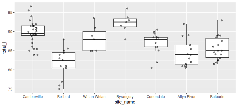
ggplot(possum_df, aes(x = site_name, y = total_l)) +
  geom_boxplot(outlier.shape = NA) +
  geom_jitter(width = 0.15, alpha = 0.5)

What the Plot Already Told Us

Before a single test:

  • Bellbird sits low
  • Byrangery sits high
  • The middle five overlap heavily
  • Boxes are about the same height — spread looks similar across sites
  • No wild outliers

So we expect: a significant overall test, driven by the ends, with the middle a mess.

Tip

🎯 Why this matters

Predicting the answer before you test is not cheating. It is the only way to notice when the output is wrong.

If the test comes back saying nothing differs, you now know to go looking for a mistake.

The Group Means

possum_df %>%
  group_by(site_name) %>%
  summarise(n = n(),
            mean_total = round(mean(total_l), 1),
            sd_total   = round(sd(total_l), 2))
# A tibble: 7 × 4
  site_name       n mean_total sd_total
  <fct>       <int>      <dbl>    <dbl>
1 Cambarville    33       89.7     2.99
2 Bellbird       13       81.8     3.9 
3 Whian Whian     7       88.1     3.35
4 Byrangery       7       92.2     2.48
5 Conondale      13       86.9     3.01
6 Allyn River    13       84.5     3.65
7 Bulburin       18       85.7     3.12

A Warning About the Obvious Story

Seven sites on a north–south gradient. Tempting story:

Colder in the south → bigger animals. Bergmann’s rule.

Look again. The two Victorian sites are the southernmost — and they are at opposite extremes:

  • Cambarville 89.7 cm
  • Bellbird 81.8 cm

Two sites, same state, 8 cm apart. Latitude cannot explain that.

Warning

⚠️ Do not let the test write your story

A significant F tells you the sites differ. It says nothing about why.

“Sites differ” is the finding. “Because of latitude” would be a second claim, and this data does not support it.

🧩 Chunk 3 of 5 · Fit the Model, Run the Test

We will cover: lm() for more than two groups, then car::Anova() and how to read its table.

Fit It With lm() — Same Function as Always

total_model <- lm(total_l ~ site_name, data = possum_df)

Note

🧠 Nothing new here

response ~ predictor, exactly as in regression. The only change is that the predictor is a factor with seven levels instead of a number.

lm() does not need a different function for ANOVA. ANOVA is a linear model. That is not a simplification — it is literally the same machinery.

Do Not Read summary() First

summary(total_model)   # six rows of "site_nameBellbird" etc.

summary() gives you six slopes, each comparing one site to Cambarville — because Cambarville is level 1, so it became the baseline.

That answers “is each site different from Cambarville?”, which is not the question. Nobody asked about Cambarville.

Warning

⚠️ The wrong table

Six p-values, all against an arbitrary reference group. Change which site is level 1 and all six change.

We want one p-value for site_name as a whole.

The Right Table: car::Anova()

Anova(total_model, type = 2)
Anova Table (Type II tests)

Response: total_l
           Sum Sq Df F value    Pr(>F)    
site_name  907.59  6  14.582 8.452e-12 ***
Residuals 1006.24 97                      
---
Signif. codes:  0 '***' 0.001 '**' 0.01 '*' 0.05 '.' 0.1 ' ' 1

Important

✅ This is the result

F(6, 97) = 14.58, p = 8.45 × 10⁻¹²

One line. One p-value. One question answered: the seven site means are not all the same.

Reading That Table

  • Sum Sq 907.6 — variation explained by site
  • Sum Sq 1006.2 — variation left over within sites
  • Df 6 — seven groups minus one
  • Df 97 — 104 possums minus 7 groups
  • F value 14.58 — the ratio, after dividing each Sum Sq by its Df
  • Pr(>F) — how often an F this big happens when nothing is going on

\(F = 14.58\) means between-site variation is 14 and a half times within-site variation.

Note

🔢 Why type = 2?

With one factor, Type I, II and III all give the identical answer. It genuinely does not matter here.

We write type = 2 anyway, as a habit, because the moment you add a second factor it starts mattering a great deal.

How Big Is It? F Does Not Tell You

effectsize::eta_squared(Anova(total_model, type = 2), partial = FALSE)
# Effect Size for ANOVA (Type II)

Parameter | Eta2 |       95% CI
-------------------------------
site_name | 0.47 | [0.34, 1.00]

- One-sided CIs: upper bound fixed at [1.00].

Eta-squared (\(\eta^2\)) = 0.47.

Which site a possum came from accounts for 47% of all the variation in total length.

The other 53% is possums being individuals.

Tip

🎯 p ≠ size

p answers “is it real?” \(\eta^2\) answers “is it big?”

With a big enough sample, a trivial difference gets a tiny p. Always report both.

🧩 Chunk 4 of 5 · Check the Assumptions

We will cover: what ANOVA assumes, why you check it after fitting, and two packages that do the work.

Two Assumptions, Checked on the Residuals

  1. Equal variances across groups — each site is about equally spread
  2. Normal residuals — what the model missed is normally distributed

Plus one you check by thinking, not testing:

  1. Independence — each possum is one animal, trapped once, measured once ✅

Important

⚠️ Order matters

You cannot check residuals before you have residuals. So:

fit first, then check.

If the check fails you go back and change the model — you do not delete the data.

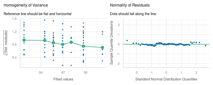
The Visual Check — check_model()

check_model(total_model, check = c("homogeneity", "qq"))

What You Are Looking For

Those are the two panels that match our two assumptions:

  • Homogeneity of variance — the line should be flat. A slope or a wedge means spread changes across groups
  • Normality of residuals — the dots should hug the diagonal

Both look healthy here. That is a boring plot, and boring is exactly what you want.

Note

📺 On your screen you get five

Plain check_model(total_model) draws all five:

  • posterior predictive check
  • linearity
  • homogeneity of variance
  • influential observations
  • normality of residuals

We asked for two here only so they fit on a slide.

If check_model() Throws an Error

Five panels need room. If the RStudio Plots pane is small, check_model() fails with a complaint about the plot size rather than drawing anything.

Two fixes:

  • Drag the Plots pane bigger and run it again, or
  • Ask for fewer panels, as we did above:
check_model(total_model,
            check = c("homogeneity", "qq"))

Warning

⚠️ Not your code

This error is about your window, not your model. Nothing is wrong with the analysis.

It catches everybody once.

The Formal Tests

# Equal variances across sites
leveneTest(total_l ~ site_name, data = possum_df)
Levene's Test for Homogeneity of Variance (center = median)
      Df F value Pr(>F)
group  6  0.5032 0.8046
      97               
# Normal residuals
shapiro.test(residuals(total_model))

    Shapiro-Wilk normality test

data:  residuals(total_model)
W = 0.98939, p-value = 0.588

Same Two Checks, Said in English

check_homogeneity(total_model)
OK: There is not clear evidence for different variances across groups (Bartlett Test, p = 0.867).
check_normality(total_model)
OK: residuals appear as normally distributed (p = 0.602).

Important

✅ Both assumptions pass

  • Levene p = 0.805 → no evidence variances differ
  • Shapiro–Wilk p = 0.588 → no evidence residuals are non-normal

High p-values are the good outcome here. You are hoping not to reject.

Careful: These Tests Are Backwards

For the main test, a small p was the interesting result.

For assumption tests it is the opposite — a small p means your test is in trouble.

That inversion catches people constantly. Say it out loud each time:

“Levene p = 0.805. Big. Variances are fine. Carry on.”

Warning

⚠️ And do not over-trust them

With small groups these tests are weak — they pass almost anything.

With huge samples they are brutal — they fail on differences too small to matter.

Look at check_model() as well, always.

🧩 Chunk 5 of 5 · Which Sites Actually Differ?

We will cover: why F is not the end, emmeans, Tukey adjustment, and reading a compact letter display.

F Said “Not All Equal” — That Is All It Said

We have F(6, 97) = 14.58, p < 0.001.

That is: at least one site differs from at least one other.

It does not tell you:

  • which sites
  • how many
  • in which direction

For that you need post-hoc comparisons — “after the fact”.

Note

🧠 Why this is allowed now

Doing 21 comparisons was wrong as a first move.

Doing them after a significant F, with the p-values adjusted, is the standard, defensible approach.

The gate came first.

Estimated Means With emmeans

site_means <- emmeans(total_model, ~ site_name)
site_means
 site_name   emmean    SE df lower.CL upper.CL
 Cambarville   89.7 0.561 97     88.6     90.8
 Bellbird      81.8 0.893 97     80.0     83.5
 Whian Whian   88.1 1.220 97     85.7     90.5
 Byrangery     92.2 1.220 97     89.8     94.7
 Conondale     86.9 0.893 97     85.2     88.7
 Allyn River   84.5 0.893 97     82.8     86.3
 Bulburin      85.7 0.759 97     84.2     87.2

Confidence level used: 0.95 

All 21 Pairs, Honestly Adjusted

pairs(site_means, adjust = "tukey")
                   contrast estimate t.ratio p.value
1    Cambarville - Bellbird     7.94    7.53 < 1e-04
2 Cambarville - Whian Whian     1.64    1.22 0.88310
3   Cambarville - Byrangery    -2.53   -1.89 0.49301
4   Cambarville - Conondale     2.79    2.64 0.12429
5 Cambarville - Allyn River     5.17    4.91 < 1e-04
6    Cambarville - Bulburin     4.02    4.26 0.00092
7    Bellbird - Whian Whian    -6.30   -4.17 0.00124
8      Bellbird - Byrangery   -10.47   -6.94 < 1e-04

Note

First 8 of 21 rows. Tukey widens every p-value to pay for running 21 tests.

The Count

Of the 21 pairs, 10 are significant and 11 are not.

Which is exactly what the boxplot predicted:

  • Everything involving Bellbird (lowest) or Byrangery (highest) tends to separate
  • The middle five mostly do not separate from each other

Twenty-one rows is a lot to read. There is a better way to show it.

Tip

🎯 Report the pattern

Nobody wants 21 p-values in a results section.

They want to know which groups cluster together. That is what letters do.

Compact Letter Display

cld(site_means, Letters = letters)
 site_name   emmean    SE df lower.CL upper.CL .group
 Bellbird      81.8 0.893 97     80.0     83.5  a    
 Allyn River   84.5 0.893 97     82.8     86.3  ab   
 Bulburin      85.7 0.759 97     84.2     87.2   b   
 Conondale     86.9 0.893 97     85.2     88.7   bc  
 Whian Whian   88.1 1.220 97     85.7     90.5   bcd 
 Cambarville   89.7 0.561 97     88.6     90.8    cd 
 Byrangery     92.2 1.220 97     89.8     94.7     d 

Confidence level used: 0.95 
P value adjustment: tukey method for comparing a family of 7 estimates 
significance level used: alpha = 0.05 
NOTE: If two or more means share the same grouping symbol,
      then we cannot show them to be different.
      But we also did not show them to be the same. 

How to Read Letters

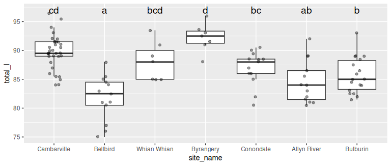
Share a letter → not shown to differ. No letter in common → differ.

  • Bellbird a — alone at the bottom
  • Allyn River ab — not distinguishable from either neighbour
  • Byrangery d — alone at the top
  • Bellbird vs Byrangery: a vs d, nothing shared → differ

A clean ladder from 81.8 cm up to 92.2 cm.

Warning

⚠️ Read R’s own note

“If two or more means share the same grouping symbol, then we cannot show them to be different. But we also did not show them to be the same.”

Sharing a letter is failure to detect a difference — not evidence of equality. Especially at Byrangery, where n = 7.

Put the Letters on the Plot

letters_df <- as.data.frame(cld(site_means, Letters = letters)) %>%
  mutate(group = trimws(.group))

ggplot(possum_df, aes(x = site_name, y = total_l)) +
  geom_boxplot(outlier.shape = NA) +
  geom_jitter(width = 0.15, alpha = 0.4) +
  geom_text(data = letters_df,
            aes(x = site_name, y = 97, label = group),
            size = 5)

Writing It Up

Important

📝 The whole result, in three sentences

Total length differed significantly among the seven trapping sites (one-way ANOVA, F(6, 97) = 14.58, p < 0.001), and site accounted for 47% of the variation in length (η² = 0.47). Residuals were normally distributed (Shapiro–Wilk p = 0.59) with homogeneous variances across sites (Levene’s test p = 0.81). Tukey-adjusted comparisons separated Bellbird (mean 81.8 cm) from Byrangery (92.2 cm), with the remaining five sites forming an overlapping middle group.

What Belongs in That Sentence

Every number has a job:

  • The test — one-way ANOVA
  • F with both df — F(6, 97); the df let a reader reconstruct your design
  • p — as p < 0.001, not p = 0
  • Effect size — η², because p alone hides size
  • Assumption checks — so the reader knows you looked
  • The pattern — which groups, in which direction, with means

Warning

⚠️ Never write “p = 0.000”

Software rounds. Probability does not reach zero.

Write p < 0.001 and move on.

Common Ways This Goes Wrong

  • Grouping variable left as a number → you fit a line through site IDs
  • Reading summary() instead of Anova() → six wrong p-values
  • Checking assumptions before fitting → there are no residuals yet
  • Expecting a small p for Levene → backwards
  • Stopping at a significant F → F never says which groups
  • Unadjusted pairwise tests → the 66% problem, straight back
  • Calling shared letters “the same” → they are undetected, not equal

Tip

🎯 The recipe, memorised

  1. factor() the groups
  2. Plot it
  3. lm()
  4. Anova(type = 2)
  5. check_model() + leveneTest()
  6. eta_squared()
  7. emmeans() → pairs() → cld()
  8. Write the sentence

Your Homework: The Same Possums, a Different Ruler

The file has four measurements on every animal. We used total_l. For homework you run the whole recipe again on tail_l — tail length.

Same 104 animals, same seven sites, same eight steps. A different ruler.

The question is whether the pattern holds: do the sites that had the longest bodies also have the longest tails?

Note

📂 What you will do

All eight steps on tail_l, then one paragraph comparing your letters to the ones we got today.

Plus one optional part where an assumption fails on purpose.

And a Preview of Next Class 🦗

Next time: New Zealand tree wētā, a large flightless cricket relative whose adult males come in three distinct forms — small-jawed sneaks, intermediates, and huge-jawed fighters.

We will find that the three forms differ enormously in ear size.

Then we will divide ear size by body size, run the identical test, and the answer will change.

Tip

🎯 Why that matters

ANOVA answers the question you asked it.

Making sure that is the question you meant is the whole job of next class.

Recap

  • Many t-tests inflate error — 7 groups, 21 pairs, 66% false-positive risk
  • ANOVA asks one question: between-group variation vs within-group variation
  • factor(levels =, labels =) turns group codes into named, ordered groups
  • lm() fits it — ANOVA is a linear model; car::Anova(type = 2) gives the one right table
  • Check after fitting — check_model(), leveneTest(), shapiro.test(); here a big p is good
  • η² says how big; F only says whether
  • emmeans() → pairs() → cld() says which — with p-values adjusted
  • Shared letters mean not shown to differ, never shown to be the same

Note

✅ Next

Open the activity and run all of it. Homework is tail_l. Next class, the wētā. 🦗