Lecture 02 — Introduction to R and Positron

R, Positron and Projects

Bill Perry

2026-09-10

Where we left off (Lecture 01)

• Science fundamentals — falsifiable predictions; null vs. alternate hypotheses
• Our class project — leaf morphology: sunny vs. shady sides of trees
• Design — randomization, replication (multiple trees), sampling limits
• Variables — dependent (leaf mass/size) vs. independent (shade of tree)
• Spreadsheet hygiene — metadata, consistent column names, units, clean sheet design
• Installed R and Positron before today

Note

✅ Key idea

Today we take that tidy spreadsheet and bring it to life in R.

Goals for today

• Get R and Positron oriented — the four panes
• Organize a project so future-you can find things
• Learn how R actually works:
  • using it as a calculator
  • storing things with <- the assignment operator - alligator eats the minus sign…
  • values, vectors, and data types
  • writing a script
• Load our tree data and make a first plot

Tip

🖐 Try it yourself

By the end you will run real code on our leaf data — not a toy dataset.

Diagram showing ggplot’s layered construction: a data frame, then an aes() mapping, then a geom, stacked with + into a finished plot.

Part 1 · Setting up

What is R, really?

• R is the engine — a free language for data and statistics
• We drive that engine through an IDE (a code editor)
• Two good IDEs — you may try both:
  • Positron — what we use (recommended)
  • RStudio — the long-time classic

Note

📖 New word

IDE = Integrated Development Environment. Think of R as the car engine and the IDE as the seat, wheel, and dashboard.

Screenshot of the Positron IDE welcome screen, showing its Console/Terminal, Variables, and Plots panes.

Organize the project before you code

Make one folder per project. Everything for the tree experiment lives together:

tree_project/
├── data/          ← your Excel and CSV files
├── scripts/       ← your .R code files
└── figures/       ← plots you save

• In Positron: File → Open Folder… and pick this folder
• Every path is then relative to the project — no more C:/Users/.../Desktop/... nightmares

Note

✅ Key idea

A tidy folder today saves an hour of “where did I put that file?” next week.

Note

📚 Reference

R for Data Science (2e), Ch. 6 — Workflow: scripts and projects. Covers exactly this: projects, relative paths, and “what is the source of truth.”

Note

📊 Coming from Excel?

• In Excel you keep one big file and it can be hard to figure out what was done and how
• In R we keep raw data untouched and
  • write new processed files
    • — so you can always trace your steps and never overwrite your original numbers

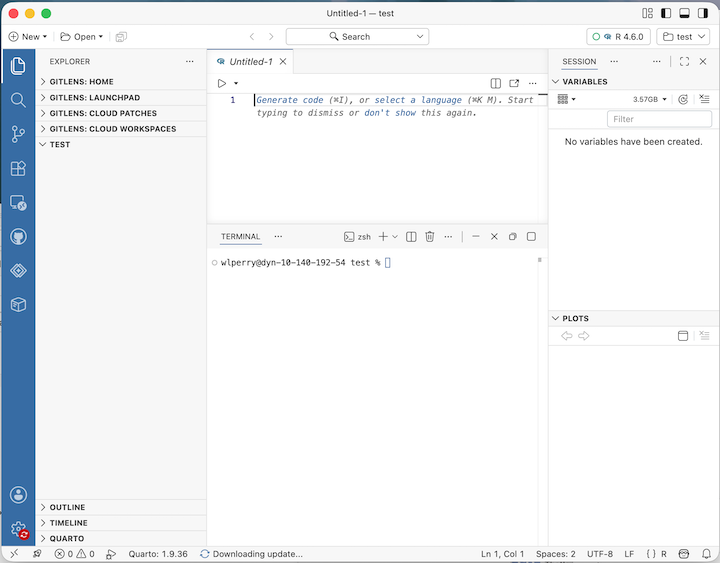
A quick tour of Positron

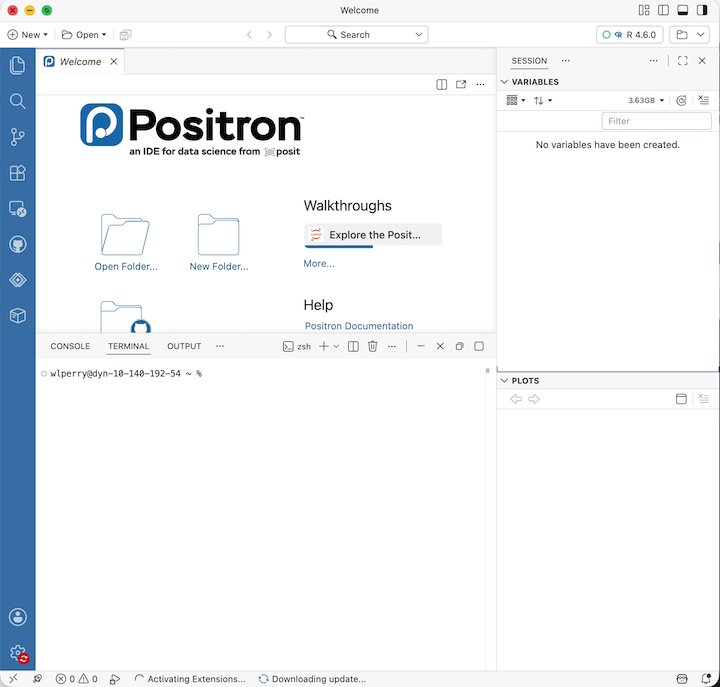
Four panes you will use constantly:

• Editor (top-left) — your scripts live here when you have a script open
• Console / Terminal (bottom) — where code runs
• Variables / Session (right) — everything you have stored
• Plots (right) — your figures appear here

Tip

🖐 Try it yourself

• Find each pane on your screen now.
• Click the Console tab — that is where we start next.

Screenshot of the Positron IDE with its Editor, Console/Terminal, Variables, and Plots panes visible.

Part 2 · How R works

R is a calculator

Type math straight into the console and press Enter:

3 + 5
12 / 7
2 ^ 10

R answers immediately. The console is great for quick “what is the answer?” questions.

Warning

⚠️ Watch out!

• A + at the start of the console line means R is still waiting for you to finish a command.
• Press Esc to start over.

Note

📊 Coming from Excel?

• This is just like typing =3+5 into an Excel cell
• except there are no cells, just a line you type and run

Storing values with <- assignment operator - alligator eats the minus sign

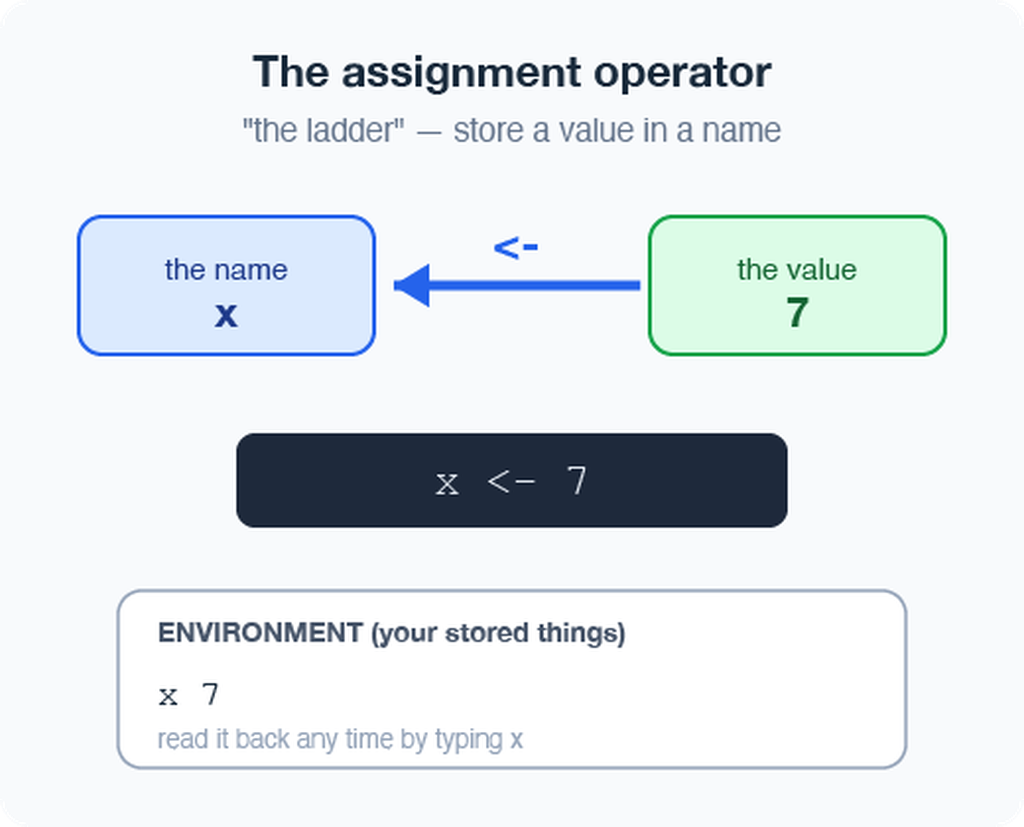
To keep a value, give it a name with the assignment operator <-:

x <- 7          # store 7 under the name x
x               # type the name to read it back
x * 2           # use it in math

• <- puts the value into your environment (look in the Variables pane!)
• Shortcut: Alt + - (Win) or Option + - (Mac) types <- for you

Note

📖 New word

Assignment operator <- “puts the thing on right and stores it in the name on left.” Do not use =

Diagram of the assignment operator: an arrow from a value (7) on the right pointing left into a name (x), with the environment then showing x storing 7.

Naming your objects well

Good names make code readable months later:

• Be explicit, not too long: leaf_mass, not x2
• Cannot start with a number — x2 ✅, 2x ❌
• R is case-sensitive — mass_g ≠ Mass_g
• Use lower_snake_case — words separated by underscores

leaf_mass   <- c(4, 3, 5, 7)   # good
LeafMass    <- c(4, 3, 5, 7)   # works but avoid
leaf.mass   <- c(4, 3, 5, 7)   # avoid dots

Warning

⚠️ Watch out!

mass_g and mass_G are two different objects. Pick one style and stick with it. I URGE you to use lower case and underscores — lower_snake_case, always.

Note

📖 New word

Object (R) = variable (Excel/other languages). Same idea: a named container that holds something.

• Our naming convention throughout this course:
  • data frames → _df
  • plots → _plot
  • models → _model

Note

📚 Reference

R for Data Science (2e), Ch. 2 — Workflow: basics (naming, calling functions) and Ch. 4 — Workflow: code style (spacing, pipes). Short chapters — worth reading both.

Leave notes with comments #

Anything to the right of # is ignored by R — it is a note for humans:

# weights of four leaves, in grams
leaf_mass <- c(4, 3, 5, 7)

mean(leaf_mass)   # average leaf mass

• Comment generously — your future self will thank you
• Shortcut to toggle: Ctrl/Cmd + Shift + C - this can be modified

Note

✅ Key idea

If a line confused you while writing it, comment why you did it.

Note

📊 Coming from Excel?

Comments are like the notes you scribble in a cell — but they never get in the way of the numbers or the code.

Functions and their arguments

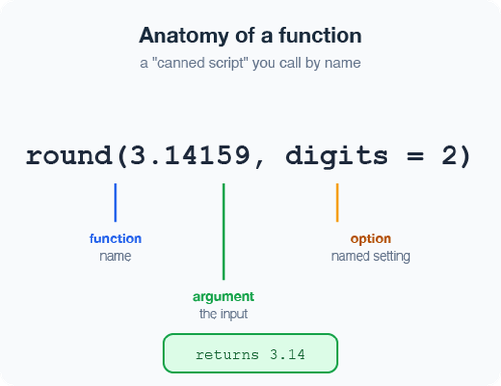
A function is a canned script you call by name. You feed it arguments (inputs); it returns a result:

sqrt(10)                         # one argument
round(3.14159)                   # default: 0 digits → 3
round(3.14159, 2)                # two digits → 3.14
round(x = 3.14159, digits = 2)  # named arguments

Stuck on a function?

?round        # open the help page
args(round)   # what arguments does it take?

Note

📖 New word

Argument = an input you hand to a function inside its ( ).

Diagram labeling the parts of round(3.14159, digits = 2): the function name, the argument (the input value), and a named option, with the returned result shown below.

Vectors — a row of values

A vector is a series of values built with c() (“combine”) or concatenated list:

mass_g <- c(4, 3, 5, 7)          # numbers
shade     <- c("sunny", "shady")     # text needs quotes

Inspect any vector:

length(mass_g)   # how many values?
class(mass_g)    # what type?
str(mass_g)      # quick structure overview

Warning

⚠️ Watch out!

Quotes matter: "sunny" is text. Without quotes, R hunts for an object named sunny and errors when it cannot find one.

Note

✅ Key idea

A vector is the workhorse of R. A spreadsheet column is really just a vector.

Data types live inside vectors

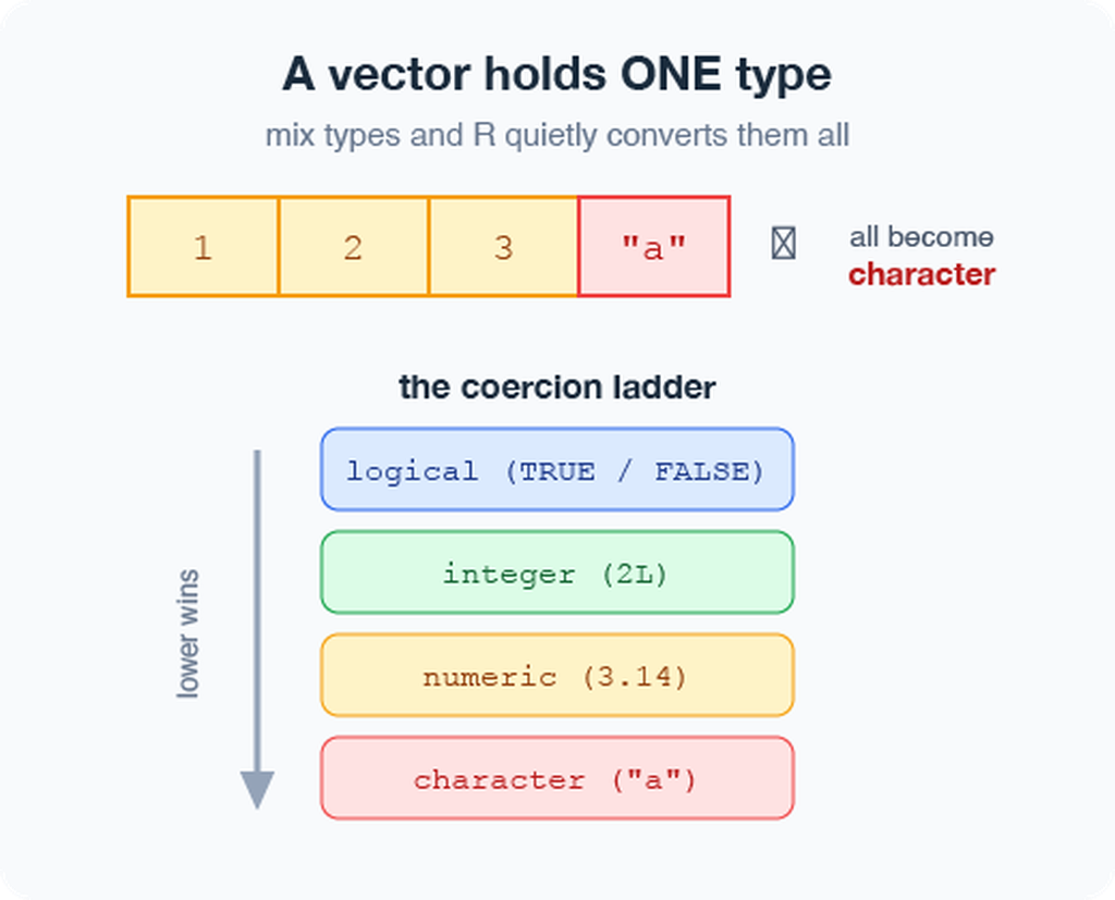
Every vector holds one type:

• numeric — 4, 3.5
• character — "sunny"
• logical — TRUE / FALSE

Mix types and R quietly coerces them all to one:

c(1, 2, 3, "a")     # all become character
c(1, 2, 3, TRUE)    # TRUE becomes 1
class(c(1, 2, 3, "a"))

Note

📖 New word

Coercion = R automatically converting everything in a vector to a single shared type.

Diagram of R data types: a vector mixing numbers and a string all coercing to character, and a coercion ladder from logical up through integer, numeric, to character.

Part 3 · From console to script

Do not retype — use a script

The console forgets and you would have to retype all of your code over and over….

A script (.R file) remembers and re-runs code

• File → New File → R File opens a blank script
• Type your commands, one per line
• Put the cursor on a line and press Ctrl/Cmd + Enter to run it
• Save with Ctrl/Cmd + S — reopen later and re-run everything

x    <- 7
y    <- 5
x + y

Note

✅ Key idea

• Console = scratch paper.
• Script = the lab notebook you keep.

Screenshot of the Positron editor pane with a script file open above the Terminal, and the Explorer, Variables, and Plots panes visible.

Packages — extending what R can do

Like apps for your phone, packages add new abilities to R.

Install once — downloads to your computer (do this in the Console, not in your script):

install.packages("tidyverse")
install.packages("readxl")
install.packages("janitor")

Load every session — activates it for today (put this at the top of every script):

library(tidyverse)   # data wrangling + plotting
library(readxl)      # read Excel files
library(janitor)      # cleans up messy column names

Warning

⚠️ Watch out!

If R says “could not find function read_excel”, you forgot the library(readxl) line.

Note

📖 New words

• Package = the installed toolbox (install once).
• Library = loading that toolbox into today’s session (every session).

Part 4 · Loading our data

Two functions for two file types

Put your files in the project’s data/ folder, then:

library(tidyverse)
library(readxl)
library(janitor)

# Excel files (.xlsx)
tree_df <- read_excel("data/2026_09_03_data_sci_leaf_area.xlsx") %>%
  clean_names()

# CSV files (.csv) — used by NOAA, iNaturalist, many databases
noaa_df <- read_csv("data/noaa_global_yearly_temps.csv") %>%
  clean_names()

Note

✅ Key idea

• read.csv() - comes with base r and can have issues
• read_excel() - needs library(readxl).
• read_csv() - needs library(tidyverse)
• clean_names() - needs library(janitor); turns messy Excel headers like "Leaf Mass (g)" into tidy names like leaf_mass_g automatically

Note

📊 Coming from Excel?

read_excel() and read_csv() are the bridge from your file into R. Your file’s first row becomes the column names in R.

Note

📚 Reference

R for Data Science (2e), Ch. 7 — Data import. Covers read_csv() in depth, including column types and messy real-world files.

Meet the data frame

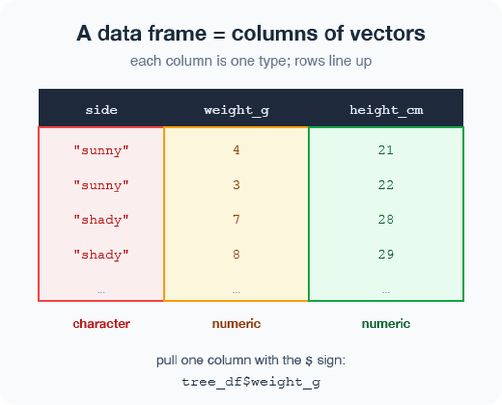
A data frame is a table: each column is a vector of one type, and the rows line up.

Our tree_df has eight columns:

• twig_id, leaf_id, teams — sample identifiers (character)
• shade — "sunny" / "shady" (character)
• mass_g, petiole_mm, thickness_mm, paper_mass_g (numeric)

Pull a single column with $:

tree_df$mass_g     # just the leaf masses, as a vector

Note

📖 New word

Data frame = R’s word for a spreadsheet-style table.

Diagram of a data frame as columns of vectors: a shade column (character), mass_g column (numeric), and petiole_mm column (numeric), with rows lining up across columns.

Look at your data before trusting it

Always eyeball a new data frame:

head(tree_df)      # first 6 rows
tail(tree_df)      # last 6 rows
dim(tree_df)       # rows, columns  → 41  8
names(tree_df)     # column names

# Tidyverse-style structure check (prefer this over str):
glimpse(tree_df)   # one line per column: name, type, first values

# Base R equivalent:
str(tree_df)       # same information, different layout

Tip

🖐 Try it yourself

Run glimpse(tree_df). How many rows? What type is shade?

Note

✅ Key idea

Check dim() and glimpse() every single time you load data. Typos and wrong column types hide here.

Warning

⚠️ Watch out!

If a number column shows as <chr>, a stray letter or comma snuck into your spreadsheet.

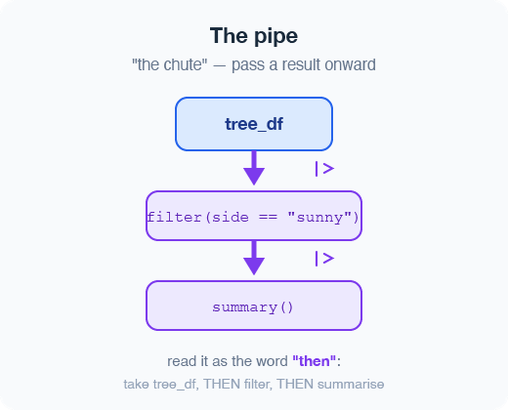
The pipe %>% — read it as “then”

The pipe sends a result straight into the next function. Read %>% as the word “then”:

# Start with simple examples:
tree_df %>% nrow()         # take tree_df, THEN count rows
tree_df %>% names()        # take tree_df, THEN list column names
tree_df %>% summary()      # take tree_df, THEN summarize

# Chain two steps:
tree_df %>%
  head(3)                  # take tree_df, THEN show first 3 rows

In Lecture 03 we will chain more steps together.

Note

📖 New word

Pipe %>% = “take what is on the left and feed it to the function on the right.”

Diagram of the pipe operator: tree_df flows down into filter(shade == “sunny”), then flows down into summary(), read as “take tree_df, then filter, then summarise.”

Note

Two pipes — same idea:

• %>% — from tidyverse (we use this one)
• |> — built into R 4.1+ (the “native pipe”)
• They behave identically for everything in this course but I prefer the %>%

Part 5 · Your first plot

ggplot: build a picture in layers

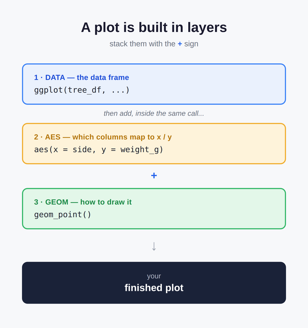
Plots are built from three core pieces, joined with +:

ggplot(tree_df, aes(x = shade, y = mass_g))

1. data — which data frame (tree_df)
2. aes — which columns map to x and y
3. geom — how to draw it (add with +)

ggplot(tree_df, aes(x = shade, y = mass_g)) +
  geom_point()

Warning

⚠️ Watch out!

• The + must sit at the end of a line, never the start.
• + at the start = error
• AND YES — it’s confusing to use %>% for code and + for plots, but that’s just how it is.

Note

📚 Reference

R for Data Science (2e), Ch. 1 — Data Visualization, and Whitlock & Schluter, Ch. 2 — Displaying Data, on why we choose one graph type over another for a given kind of data.

Diagram showing ggplot’s layered construction: a data frame, then an aes() mapping, then a geom, stacked with + into a finished plot — reused here for building your first plot.

Improve it one layer at a time

Since shade is a category, a boxplot with the raw points on top tells the story well:

# define the point position ONCE, at the top, so every layer can reuse it
jitter_pos <- position_jitter(width = 0.15, seed = 42)

ggplot(tree_df, aes(x = shade, y = mass_g)) +
  geom_boxplot() +
  geom_point(position = jitter_pos, alpha = 0.6, color = "tomato") +
  labs(x = "Side of tree",
       y = "Leaf mass (g)",
       title = "Sunny vs. shady leaves")

Tip

🖐 Try it yourself

Swap mass_g for thickness_mm. What changes? Try geom_violin() instead of geom_boxplot().

Before you run it: sketch what you expect this plot to look like — boxes, dots, axes — then compare it to what R draws.

Note

Why position_jitter() in a variable?

geom_point() alone stacks every leaf on one vertical line. position_jitter(width = 0.15) nudges them sideways so you can see each one; seed = 42 keeps that random nudge identical every time you render. Storing it in jitter_pos means the next layer (a mean, an error bar, a connecting line) can sit at the exact same spot.

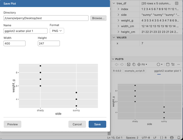
Save your plot and your script

Store the plot in an object, then save it as a PNG:

leaf_plot <- ggplot(tree_df, aes(x = shade, y = mass_g)) +
  geom_boxplot()

# Save to the figures/ folder — always use PNG, dpi = 300
ggsave("figures/leaf_mass.png",
       plot   = leaf_plot,
       width  = 6,
       height = 6,
       units  = "in",
       dpi    = 300)

• 📖 File format tip
• Save figures as PNG (.png) for reports and Canvas submissions.
• dpi = 300 means 300 dots per inch — high enough for print and posters.

Warning

⚠️ Watch out!

ggsave() wants the filename first, then plot =. Also: dpi = 300 is publication quality — always use it.

Note

Screenshot of the Save Plot dialog in Positron’s Plots pane, with the leaf mass boxplot ready to save as a PNG.

Wrap-up · What you can now do

• Set up R + Positron and organize a project folder
• Use R as a calculator and store values with <-
• Write and run a script, with # comments
• Call functions and read their help with ?
• Build vectors, know their types
• Load Excel and CSV data with read_excel() and read_csv()
• Inspect a data frame with glimpse(), head(), dim()
• Use the pipe %>% to chain steps
• Make and save a first ggplot as a PNG

Tip

🖐 Before next class

Load tree_df, run glimpse(), and make one plot of petiole_mm by shade. Save it to figures/.

Note

✅ Key idea

You went from a blank console to a saved figure of our data. That is the whole workflow in miniature.

Up next — Lecture 03 & 04 (Week 2):

• Two lectures on ggplot2 in depth — stat_summary(), facet_wrap()/facet_grid(), scale_color_manual(), coord_cartesian(), and themes
• We will keep using our own leaf data the whole time

→ ACTIVITY 2 starts now

🛑 Go to Activity 2 — “Introduction to R and Positron”

Open the Activity 2 worksheet and work through it at your own pace, typing every code chunk into your own script in Positron. It repeats everything on these slides, in the same order, with blanks for you to fill in. Raise your hand if you get stuck — that is expected and normal.

Suggested reading before Lecture 03

• R for Data Science (2e), Ch. 1 — Data Visualization (read fully this time — you skimmed it before Lecture 02)
• R for Data Science (2e), Ch. 6 — Workflow: scripts and projects, if you have not read it yet
• Whitlock & Schluter, Ch. 2 — Displaying Data

Note

Both books are in the course readings/ folder.

Getting unstuck

When code breaks (it will — that is normal):

• ?function_name — the built-in help page
• Read the error message out loud; it usually names the line
• Check: did you load library(tidyverse) and library(readxl)?
• Check: spelling? A missing ) or +?
• The posit/tidyverse cheatsheets are excellent: posit.co/resources/cheatsheets
• Bring the exact error (copy-paste it) to class or office hours

Note

✅ Key idea

Every coder googles error messages daily. Getting stuck is not failing — it is the job. Your job is to learn, and learning means breaking things and figuring out why.

Note

📊 Coming from Excel?

In Excel you fix errors by clicking around. In R you fix them by reading the message and editing one line. Slower at first, far more powerful soon.