Lecture 11 — One-Way ANOVA: Comparing Many Groups

Partitioning variance, checking assumptions, and post-hoc tests with emmeans

Bill Perry

2026-07-05

Where we left off (Lecture 10)

Factors — categorical variables with an ordered set of levels
fct_reorder() / fct_relevel() — set the order and the reference group
Cleaner, better-ordered plots for grouped data

Note

✅ Transition

The t-test (Lecture 04) compared two groups. But biology is full of three-or-more group questions — three species, four sites, five treatments. Now that you can control factor levels, today we learn the test for many groups: one-way ANOVA.

Goals for today

Understand why we don’t just run many t-tests
See how the F-statistic compares between- vs within-group variance
State ANOVA hypotheses (H₀: all means equal)
Check assumptions — normality of residuals, equal variance
Run it two ways: aov() and car::Anova()
Find which groups differ with emmeans post-hoc tests

Tools today:

palmerpenguins, tidyverse
car — Levene’s test, Anova()
emmeans, multcomp — post-hoc

Textbook:

📖 Whitlock & Schluter, Ch. 15 — ANOVA
📖 R4DS Ch. 16 — Factors
📖 R4DS Ch. 9 — Layers

Naming: models → _model, plots → _plot

How to Use These Slides — Predict · Type · Run

This lecture runs in four short chunks. After each chunk you switch to the activity and type the code yourself.

For every code block, do three things:

Predict — before it runs, say what you think the output will be
Type it out by hand — do not copy-paste
Run it and compare to your prediction

Note

✅ Why bother? (the evidence)

Predicting first forces you to retrieve what you know — the gap between guess and answer is what makes it stick.
Typing by hand builds the finger-memory and error-spotting that copy-paste skips.
Chunk → immediate practice keeps each idea in working memory long enough to form a lasting schema.

🧩 Chunk 1 of 4 · Why ANOVA & the F-Statistic

We will cover: why not many t-tests, what ANOVA asks, how F partitions variance, and a first look at the penguin data.

Tip

🖐 After this chunk: Activity Parts 1–3 (load the penguins, explore, state hypotheses).

Why Not Just Run Many t-Tests?

With 3 groups you’d need 3 t-tests (A–B, A–C, B–C). With 4 groups, 6 tests.

Every test at α = 0.05 has a 5% chance of a false positive. Run several and those risks stack up:

3 tests → ~14% chance of at least one false positive
6 tests → ~26%

ANOVA asks the question once, holding the overall error rate at 0.05.

Important

The multiple-comparisons problem

More tests = more chances to be fooled by noise. ANOVA is the single, honest test for “do any of these groups differ?”

📖 W&S §15.1 — why a single test

What One-Way ANOVA Asks

One numeric response (Y) across the levels of one categorical predictor (X).

	Hypothesis
H₀ — null	all group means are equal (\(\mu_1 = \mu_2 = \mu_3\))
Hₐ — alternate	at least one group mean differs

Note what Hₐ does not say: it does not tell you which group differs — that comes later, from the post-hoc test.

Our question today:

Do the three penguin species differ in body mass?

Y = body_mass_g
X = species (Adelie, Chinstrap, Gentoo)

The F-Statistic — Between vs. Within

\[F = \frac{\text{variance BETWEEN groups}}{\text{variance WITHIN groups}}\]

Between — how far apart the group means are
Within — how much the individuals scatter inside each group

Big F → the groups are far apart relative to their internal noise → small p-value.

F ≈ 1 → the spread between groups is no bigger than the spread within them → no real difference.

Note

✅ Key idea

ANOVA is a signal-to-noise ratio. The “signal” is the gap between group means; the “noise” is the within-group scatter.

📖 W&S §15.1–15.2

Meet the Data — Palmer Penguins

# Load packages at the top — always -------------------
library(tidyverse)      # wrangling + ggplot2
library(palmerpenguins) # the penguins data
library(car)            # Levene's test, Anova()
library(emmeans)        # post-hoc pairwise tests

# Drop rows missing mass or species -------------------
penguins_df <- penguins %>%
  drop_na(body_mass_g, species)

penguins_df %>% count(species)

# A tibble: 3 × 2
  species       n
  <fct>     <int>
1 Adelie      151
2 Chinstrap    68
3 Gentoo      123

Three species, one lab: body mass (g) of penguins at Palmer Station, Antarctica.

drop_na() removes rows with missing mass
count(species) shows the sample size per group

Important

The groups are unbalanced (different n per species) — that matters when we pick our ANOVA type later.

Explore First — Boxplot by Species

Note

🔮 Predict first: Before the plot renders — do you expect all three species to differ, or just one? Which species do you think is heaviest?

mass_box_plot <- penguins_df %>%
  ggplot(aes(x = species, y = body_mass_g, fill = species)) +
  geom_boxplot(alpha = 0.5, outlier.shape = NA) +
  geom_point(
    position = position_jitter(width = 0.15, seed = 42),
    alpha = 0.3, size = 1.5
  ) +
  labs(x = "Species", y = "Body Mass (g)") +
  theme_minimal() +
  theme(legend.position = "none")

mass_box_plot

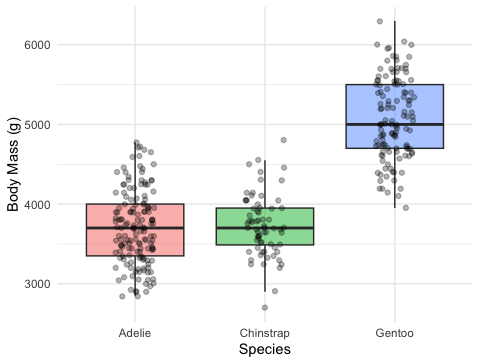
Always plot before you test.

The picture usually tells the story before the p-value confirms it
Look for separation between boxes and roughly similar spread

📖 R4DS §9 — Layers

🛑 Pause — Do Activity Parts 1–3 Now

Load the penguins, plot body mass by species, and write your hypotheses. Predict which species differ before you run anything.

🧩 Chunk 2 of 4 · Fit the Model & Check Assumptions

We will cover: fitting the model, then checking normality of the residuals and equal variance across groups.

Tip

🖐 After this chunk: Activity Parts 4–6 (fit, QQ + Shapiro on residuals, Levene’s test).

Fit the Model

# ANOVA is a linear model with a categorical X ---------
mass_model <- lm(body_mass_g ~ species, data = penguins_df)

lm(Y ~ X) — the same syntax as regression (Lecture 06)
When X is categorical, that linear model is a one-way ANOVA
We check assumptions on this model before reading any p-value

Note

✅ Key idea

ANOVA and regression are the same machinery (lm). ANOVA just has a grouping variable instead of a numeric one.

📖 W&S §15.2

Assumption 1 — Normality of the Residuals

# QQ plot of residuals — points should track the line -
qq_mass_plot <- penguins_df %>%
  mutate(resid = residuals(mass_model)) %>%
  ggplot(aes(sample = resid)) +
  stat_qq() +
  stat_qq_line(color = "red", linewidth = 0.8) +
  labs(x = "Theoretical", y = "Sample residuals") +
  theme_minimal()

qq_mass_plot

shapiro.test(residuals(mass_model))


    Shapiro-Wilk normality test

data:  residuals(mass_model)
W = 0.99166, p-value = 0.05118

Check normality of the residuals, not the raw masses
The QQ plot is the main tool; Shapiro-Wilk is a formal check

Important

Large-sample caution: with ~340 birds, Shapiro-Wilk flags tiny departures as “significant.” Trust the QQ plot — if points track the line, you’re fine.

Assumption 2 — Equal Variance (Levene’s Test)

Note

🔮 Predict first: Look back at the boxplot spreads. Predict — will Levene’s test call the variances equal (p > 0.05) or unequal?

# Levene's test — H0: all groups have equal variance --
leveneTest(body_mass_g ~ species, data = penguins_df)

Levene's Test for Homogeneity of Variance (center = median)
       Df F value   Pr(>F)   
group   2  5.1203 0.006445 **
      339                    
---
Signif. codes:  0 '***' 0.001 '**' 0.01 '*' 0.05 '.' 0.1 ' ' 1

p > 0.05 → variances similar → classic ANOVA is fine
p < 0.05 → variances differ → use Welch’s ANOVA:

oneway.test(body_mass_g ~ species,
            data = penguins_df,
            var.equal = FALSE)

Same spirit as Welch’s t-test — robust when spreads differ.

🛑 Pause — Do Activity Parts 4–6 Now

Fit lm(body_mass_g ~ species), check the residual QQ plot + Shapiro, and run Levene’s test. Predict each result before you run it.

🧩 Chunk 3 of 4 · Run the ANOVA & Read the F Table

We will cover: the ANOVA table two ways — base aov() and car::Anova() — and why the difference matters for unbalanced data.

Tip

🖐 After this chunk: Activity Parts 7–8 (run both, read F / df / p).

Run the ANOVA — `aov()` and `summary()`

Note

🔮 Predict first: The boxplot looked very separated. Predict the p-value — closer to 0.5, 0.05, or far below 0.001?

# Classic ANOVA table (Type I sums of squares) --------
mass_aov <- aov(body_mass_g ~ species, data = penguins_df)
summary(mass_aov)

             Df    Sum Sq  Mean Sq F value Pr(>F)    
species       2 146864214 73432107   343.6 <2e-16 ***
Residuals   339  72443483   213698                   
---
Signif. codes:  0 '***' 0.001 '**' 0.01 '*' 0.05 '.' 0.1 ' ' 1

Reading the table:

Column	Meaning
`Df`	groups − 1, and residual df
`F value`	between ÷ within variance
`Pr(>F)`	the p-value for H₀

p < 0.05 → reject H₀ → at least one species differs. But which? Chunk 4.

Live Demo — Watch It Break (on purpose)

For unbalanced data we prefer car::Anova(). I’ll reach for it but type lowercase, and forget the package:

anova(mass_model)        # base R — Type I, one model at a time
Anova(mass_model)        # capital A — but car isn't loaded!

R stops:

Error in Anova(mass_model) :
  could not find function "Anova"

The fix — load car, and mind the capital A:

library(car)
Anova(mass_model, type = "II")

Tip

✅ Why show a broken run?

anova() (base) and Anova() (car) are different functions — lowercase compares models with Type I sums of squares; capital-A gives the Type II/III table you want. “could not find function” almost always means a missing library().

`car::Anova()` — Type II for Unbalanced Data

# Type II sums of squares — the right call here -------
Anova(mass_model, type = "II")

Anova Table (Type II tests)

Response: body_mass_g
             Sum Sq  Df F value    Pr(>F)    
species   146864214   2  343.63 < 2.2e-16 ***
Residuals  72443483 339                      
---
Signif. codes:  0 '***' 0.001 '**' 0.01 '*' 0.05 '.' 0.1 ' ' 1

Why Type II?

Our groups have different n (unbalanced)
With one predictor the F is the same, but Type II is the habit you want before you meet two-way ANOVA, where the type genuinely changes the answer

Note

anova() = Type I (order-dependent). Anova(type = "II") = order-independent.

🛑 Pause — Do Activity Parts 7–8 Now

Run aov() + summary(), then car::Anova(type = "II"). Predict the F and p before you read them, and confirm both tables agree.

🧩 Chunk 4 of 4 · Which Groups Differ? Post-Hoc with emmeans

We will cover: ANOVA says “some differ” — emmeans says which, with the comparisons properly adjusted.

Tip

🖐 After this chunk: Activity Parts 9–11 (pairwise tests, letters, plot, report).

Post-Hoc — Pairwise Comparisons with emmeans

Note

🔮 Predict first: From the boxplot, predict — will all three species differ from each other, or will two be statistically tied?

# Estimated marginal means + Tukey-adjusted pairs -----
mass_emm <- emmeans(mass_model, pairwise ~ species)

mass_emm$contrasts

 contrast           estimate   SE  df t.ratio p.value
 Adelie - Chinstrap    -32.4 67.5 339  -0.480  0.8807
 Adelie - Gentoo     -1375.4 56.1 339 -24.495 <0.0001
 Chinstrap - Gentoo  -1342.9 69.9 339 -19.224 <0.0001

P value adjustment: tukey method for comparing a family of 3 estimates

Reading it:

emmeans(..., pairwise ~ species) gives each group’s mean and every pairwise comparison
The p-values are Tukey-adjusted — they already correct for multiple comparisons, so the family-wise error stays at 0.05

📖 W&S §15.4 — planned vs. unplanned comparisons

Compact Letter Display — Who Shares a Letter?

# Groups that SHARE a letter are NOT different --------
multcomp::cld(mass_emm$emmeans, Letters = letters)

 species   emmean   SE  df lower.CL upper.CL .group
 Adelie      3701 37.6 339     3627     3775  a    
 Chinstrap   3733 56.1 339     3623     3843  a    
 Gentoo      5076 41.7 339     4994     5158   b   

Confidence level used: 0.95 
P value adjustment: tukey method for comparing a family of 3 estimates 
significance level used: alpha = 0.05 
NOTE: If two or more means share the same grouping symbol,
      then we cannot show them to be different.
      But we also did not show them to be the same.

How to read letters:

Same letter → not significantly different
Different letters → significantly different

This is the compact summary you see in published figures — one letter above each bar.

Tip

Install once: install.packages("multcomp")

Plot the Result — Means ± CI

mass_emm_plot <- as.data.frame(mass_emm$emmeans) %>%
  ggplot(aes(x = species, y = emmean, color = species)) +
  geom_point(size = 3) +
  geom_errorbar(
    aes(ymin = lower.CL, ymax = upper.CL),
    width = 0.15, linewidth = 0.9
  ) +
  labs(x = "Species", y = "Estimated mean mass (g)") +
  theme_minimal() +
  theme(legend.position = "none")

mass_emm_plot

Estimated marginal means with 95% confidence intervals.

Non-overlapping intervals hint at real differences
Pair this plot with the letters for a publication-ready figure

The emmeans plot is the ANOVA cousin of Lecture 03’s mean ± SE plot.

How to Report an ANOVA

# Pull the F table values for reporting ---------------
mass_tab <- Anova(mass_model, type = "II")
mass_tab

Anova Table (Type II tests)

Response: body_mass_g
             Sum Sq  Df F value    Pr(>F)    
species   146864214   2  343.63 < 2.2e-16 ***
Residuals  72443483 339                      
---
Signif. codes:  0 '***' 0.001 '**' 0.01 '*' 0.05 '.' 0.1 ' ' 1

“Body mass differed significantly among the three penguin species (one-way ANOVA: F(2, 339) = 343.6, p < 0.001). Tukey-adjusted comparisons showed all three species differed, with Gentoo heaviest and Adelie lightest.”

Always include:

Test type (one-way ANOVA)
F, both df, and the p-value
The post-hoc result (which groups differ)
Group means ± SE or CI

Never write “p = 0.000” — use “p < 0.001”.

🛑 Pause — Do Activity Parts 9–11 Now

Run the emmeans pairwise test, get the letters, plot the means ± CI, and write your results sentence. Predict which species differ before you run the comparisons.

What We Learned Today

Concepts:

Many t-tests inflate the false-positive rate — ANOVA asks once
F = between-group ÷ within-group variance (signal ÷ noise)
Assumptions: normal residuals, equal variance (Levene)
ANOVA rejects H₀ for the group, but post-hoc finds which pairs differ
Tukey adjustment keeps the family-wise error at 0.05

R skills:

lm(Y ~ group) and aov() + summary()
car::Anova(model, type = "II")
leveneTest(), shapiro.test(residuals())
emmeans(model, pairwise ~ group) + multcomp::cld()

References:

📖 W&S Ch. 15 — ANOVA
📖 R4DS Ch. 16 — Factors
📖 emmeans vignettes

Up next — Lecture 12:

Joins — combine two tables on a shared key
The prerequisite for bigger datasets — and for maps

Lecture 11 — One-Way ANOVA: Comparing Many Groups

Where we left off (Lecture 10)

Goals for today

How to Use These Slides — Predict · Type · Run

🧩 Chunk 1 of 4 · Why ANOVA & the F-Statistic

Why Not Just Run Many t-Tests?

What One-Way ANOVA Asks

The F-Statistic — Between vs. Within

Meet the Data — Palmer Penguins

Explore First — Boxplot by Species

🛑 Pause — Do Activity Parts 1–3 Now

🧩 Chunk 2 of 4 · Fit the Model & Check Assumptions

Fit the Model

Assumption 1 — Normality of the Residuals

Assumption 2 — Equal Variance (Levene’s Test)

🛑 Pause — Do Activity Parts 4–6 Now

🧩 Chunk 3 of 4 · Run the ANOVA & Read the F Table

Run the ANOVA — aov() and summary()

Live Demo — Watch It Break (on purpose)

car::Anova() — Type II for Unbalanced Data

🛑 Pause — Do Activity Parts 7–8 Now

🧩 Chunk 4 of 4 · Which Groups Differ? Post-Hoc with emmeans

Post-Hoc — Pairwise Comparisons with emmeans

Compact Letter Display — Who Shares a Letter?

Plot the Result — Means ± CI

How to Report an ANOVA

🛑 Pause — Do Activity Parts 9–11 Now

What We Learned Today

Run the ANOVA — `aov()` and `summary()`

`car::Anova()` — Type II for Unbalanced Data