Paper Calibration Curve: Predicting Leaf Area from Mass

The same analysis as regression_analysis_script.R — but as a report

Your Name Here

2026-07-05

Introduction

To estimate leaf surface area without a leaf-area meter, we built a calibration curve. Paper of uniform stock has a constant area-per-gram, so the mass of a paper square is a near-perfect linear predictor of its area. Once we know that relationship, we can trace a leaf onto the same paper, weigh the tracing, and convert its mass to area.

• Explanatory variable (X): paper mass (g) — easy to measure on a balance
• Response variable (Y): paper area (cm²) — what we want to predict

Methods

We weighed 118 paper squares of known area (1–567 cm²) and fit a simple linear regression, area_cm2 ~ mass_g, with lm(). We checked the four regression assumptions using a residuals-vs-fitted plot and a normal Q–Q plot with a Shapiro–Wilk test on the residuals. All work was done in R with the tidyverse; this report was written in Quarto so every number and figure below is computed directly from the data.

Results

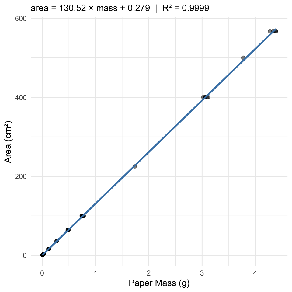
Paper mass was an extremely strong predictor of paper area (linear regression: F(1, 116) = 7.849329^{5}, p < 5^{-224}, R² = 0.9999). The calibration equation was:

\[\widehat{\text{area}} = 130.52 \times \text{mass} + 0.279\]

In words, every additional gram of paper corresponds to about 130.5 cm² of area.

Notice that F, p, R², the slope, and the intercept above were never typed by hand — they are inserted with inline code like 130.52. Change the data file and re-render, and every one of these updates itself. That is the difference from the .R script, where you would copy each number into Word yourself.

The calibration curve

Figure 1. Paper area vs. mass with the least-squares line and 95% confidence band.

Assumption checks

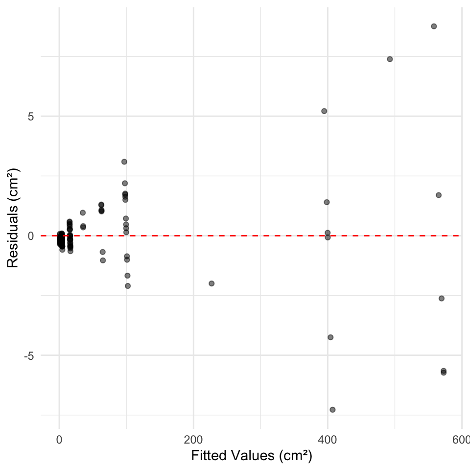
Figure 2. Residuals vs. fitted values — a random band with no funnel or curve supports linearity and equal variance.

A Shapiro–Wilk test on the residuals gave W = 0.677, p = 9.4^{-15}.

Predicting leaf area

Applying the equation to two example tracings, a sunny-side tracing of 0.092 g predicts an area of 12.3 cm², while a heavier shady-side tracing of 0.138 g predicts 18.3 cm² — consistent with our earlier finding that shady leaves are larger.

Discussion

Write one short paragraph here. Did the calibration fit well (look at R² and Figure 1)? Did the residual plot and Shapiro–Wilk support the assumptions? Why is working in area (cm²) more biologically meaningful than raw mass (g) when comparing sunny and shady leaves? This is where you paste the results paragraph you drafted in the worksheet.

References

• Whitlock, M. & Schluter, D. The Analysis of Biological Data (2nd ed.), Ch. 17.
• Wickham, H. R for Data Science (2nd ed.) — https://r4ds.hadley.nz/