Lecture 06 — Linear Regression

Predicting leaf area from paper tracing mass (Whitlock & Schluter Ch. 17)

Bill Perry

2026-07-05

Where we left off (Lecture 05)

Quarto — one .qmd file holds your writing and your code, and renders to Word, HTML, or PowerPoint
Three ingredients — YAML front matter, Markdown text, and named code chunks
Reproducibility — numbers and figures are computed, never copied by hand; change the data, press Render
Inline code — drop a live result straight into a sentence with `r `
Word reports — format: docx with toc and number-sections gives a professional document
Carried forward (Lecture 04) — shady leaves were significantly heavier than sunny leaves (Welch’s t-test, p < 0.001)

Note

✅ Transition

You can now build a reproducible report. Today’s analysis — a calibration curve that converts leaf weight into a more meaningful measurement, leaf surface area (cm²) — is the perfect thing to write up in one. The activity gives you this same analysis as both a plain .R script and a Quarto report, so you can feel the difference.

Goals for Today

Understand what linear regression does and when to use it
Learn the equation: \(\hat{Y} = a + bX\)
- slope b, intercept a, residuals, R²
Understand least squares — what the line minimizes
Fit a model in R with lm() and read every line of summary()
Apply it: build a calibration curve to predict leaf area from paper tracing mass
Check all four assumptions of regression
Use predict() to make predictions with intervals
Use mutate() to add model results to a data frame

Tip

🖐 Try it yourself

By the end you will predict leaf area from a tracing weight.

Tools today:

readxl, tidyverse

Textbook:

📖 Whitlock & Schluter Analysis of Biological Data 2nd ed.
Chapter 17 — Regression (pp. 539–575)
- §17.1 Linear regression
- §17.3 Testing slope hypotheses
- §17.4 R²
- §17.5 Assumptions

Naming conventions:

models → _model
plots → _plot

How to Use These Slides — Predict · Type · Run

This lecture runs in four short chunks. After each chunk you switch to the activity and type the code yourself.

For every code block, do three things:

Predict — before it runs, say what you think the output will be
Type it out by hand — do not copy-paste
Run it and compare to your prediction

Note

✅ Why bother? (the evidence)

Predicting first forces your brain to retrieve what it knows — the gap between guess and answer is what makes it stick.
Typing by hand builds the finger-memory and error-spotting that copy-paste skips.
Chunk → immediate practice keeps a new idea in working memory long enough to form a lasting schema.

🧩 Chunk 1 of 4 · What Regression Is

We will cover: the calibration idea, the equation \(\hat{Y}=a+bX\), least squares, R², and the four assumptions.

Tip

🖐 After this chunk: Activity Parts 1–3 (load, inspect, and scatter-plot the paper data).

Our Calibration Idea

The problem: measuring leaf surface area without a leaf area meter.

The solution — a calibration curve:

Cut paper squares of known area (1, 4, 16 … 567 cm²)
Weigh each square on a precision balance
Fit a regression line: area ~ mass
Trace a leaf on the same paper, weigh the tracing
Plug the tracing mass into the equation → predicted leaf area

Why does this work?

Paper of uniform stock has constant area density (cm² per gram). Mass and area are therefore perfectly linearly related within a sheet.

Known area (cm²)	n replicates
1	25
4	32
16	24
36	3
64	7
100	14
225–567	12

Total: 118 paper squares weighed

📖 W&S §17.1, Example 17.1 (the same logic: measure X to predict Y)

What Is Linear Regression?

Linear regression draws the best straight line through a scatter of points to predict a response variable (Y) from an explanatory variable (X).

Two key roles:

Role	Variable	Our example
Explanatory (X)	on the x-axis; what you measure	`mass_g`
Response (Y)	on the y-axis; what you want to predict	`area_cm2`

X is often something easy to measure; Y is what you actually want to know. Regression gives you the equation to convert X → Y.

📖 W&S §17.1 p. 540–541

When to use regression:

You have two numeric variables
One variable can reasonably predict or cause the other
You want an equation to make predictions for new observations

Regression vs. our t-test (Lecture 04):

Test	Question
t-test	Do two group means differ?
Regression	Does X predict Y numerically?

Regression produces a predictive equation. The t-test produces a decision about group means.

The Regression Equation

Population model (W&S §17.1):

\[Y = \alpha + \beta X + \varepsilon\]

Sample estimate (what R calculates):

\[\hat{Y} = a + bX\]

Symbol	Name	Meaning
\(\hat{Y}\)	predicted Y	estimated mean area at a given mass
a	intercept	predicted Y when X = 0
b	slope	change in Y per 1-unit increase in X
\(\varepsilon\)	residual	observed − predicted

Our equation will be: \[\widehat{\text{area}} = a + b \times \text{mass\_g}\]

Interpreting the slope:

b = the change in area (cm²) for every additional 1 gram of paper

Since 1 g ≈ 130 cm² of paper, the slope is the area density of the paper stock.

Interpreting the intercept:

a = predicted area when mass = 0

Physically this should be 0 (no paper, no area). Small non-zero values reflect measurement error.

📖 W&S §17.1 pp. 543–545

Residuals and Least Squares

Residual for observation i:

\[e_i = Y_i - \hat{Y}_i = \text{observed} - \text{predicted}\]

The least-squares line minimizes the sum of squared residuals:

\[\text{minimize} \sum_{i=1}^{n}(Y_i - \hat{Y}_i)^2\]

Squaring serves two purposes:
- - Makes all deviations positive (no cancellation)
- - Penalizes large deviations more than small ones
There is only one line that achieves this minimum — it is unique.
📖 W&S §17.1 p. 542 (Figure 17.1-2)

Visual intuition:

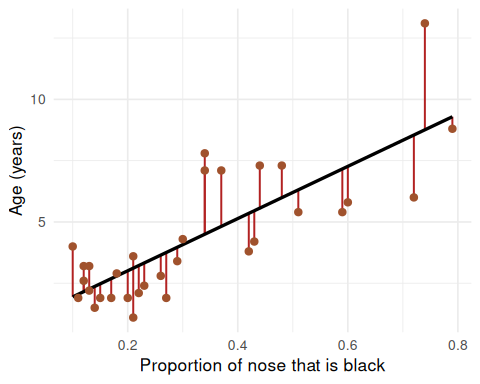
Each data point has a vertical residual — the distance from the point to the regression line.

observed Y │     ●  ← residual (positive)
           │     |
predicted Ŷ│-----●--- regression line
           │
           └──────────── X

A point above the line has a positive residual. A point below has a negative residual. The sum of all residuals = 0.

R² — How Much Does X Explain?

Note

🔮 Predict first: Paper of uniform stock has constant area-per-gram. Before you see any output, predict: will R² be near 0, 0.5, or 1?

\[R^2 = \frac{SS_\text{regression}}{SS_\text{total}} = 1 - \frac{SS_\text{residual}}{SS_\text{total}}\]

SS_total = total variation in Y around its mean
SS_regression = variation explained by X
SS_residual = variation not explained (scatter around the line)

R² ranges from 0 to 1:

R²	Interpretation
1.00	X explains all variation in Y
0.85	X explains 85% of variation
0.00	X explains nothing

📖 W&S §17.4 p. 555

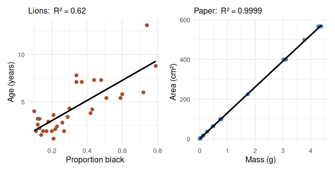
Our calibration data:

Because paper has uniform density, mass and area are nearly perfectly linearly related.

We expect R² ≈ 1.00.

Important: R² tells you how well the line fits the data you have. It does not by itself tell you whether the relationship is statistically significant — that requires a test of the slope.

A significant slope with a low R² is possible (weak but real relationship). In biology, R² values of 0.3–0.7 are common and meaningful.

Assumptions of Regression

Four assumptions must hold for the p-value and confidence intervals to be valid (W&S §17.5):

#	Assumption	How to check
1	Linearity — Y changes linearly with X	Residual vs. fitted plot
2	Independence — observations are independent	Study design
3	Equal variance — spread of residuals is constant	Residual vs. fitted plot
4	Normality — residuals are normally distributed	QQ plot + Shapiro-Wilk

Important

Check residuals, not raw data.

The normality assumption is about the residuals (observed − predicted), not the original Y values.

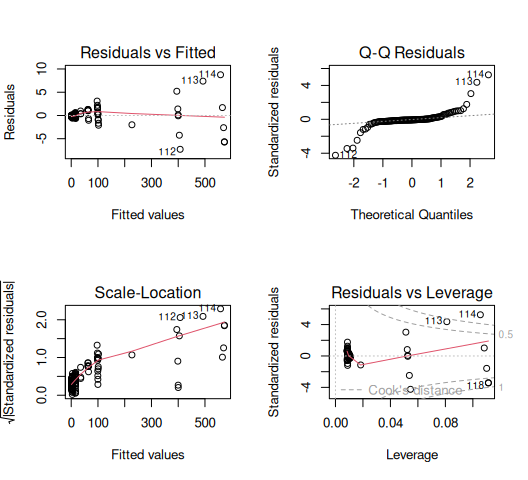
A well-fitted residual plot looks like a random horizontal cloud of points centered at zero — no curves, no funnel shapes.

📖 W&S §17.5 pp. 557–560 (Figures 17.5-1, 17.5-4)

🛑 Pause — Do Activity Parts 1–3 Now

Load paper_area_weights.xlsx, inspect it with skim(), and make the scatter of area vs mass. Predict the shape before you plot it.

🧩 Chunk 2 of 4 · Fit the Model & Read It

We will cover: loading the data, lm(), and reading every line of summary() — slope, intercept, and R².

Tip

🖐 After this chunk: Activity Parts 4–7 (fit lm(), decode summary(), pull the equation and R²).

Load Libraries and Data

# Load packages at the top of the script ---------------
library(readxl) # reading Excel files
library(tidyverse) # data manipulation + ggplot2
library(skimr) # fast data overview

# Load the paper calibration data ----------------------
paper_df <- read_excel("data/paper_area_weights.xlsx")

Note

The file paper_area_weights.xlsx contains 118 paper squares of known area (1–567 cm²) with their measured masses. This is the calibration dataset we use to predict leaf area from a tracing weight.

Inspect the Data

# Quick overview of the calibration data ---------------
skim(paper_df)

Data summary
Name	paper_df
Number of rows	118
Number of columns	2
_______________________
Column type frequency:
numeric	2
________________________
Group variables	None

Variable type: numeric

skim_variable	n_missing	complete_rate	mean	sd	p0	p25	p50	p75	p100	hist
area_cm2	0	1	71.64	144.46	1	4.00	16.00	64.00	567.00	▇▁▁▁▁
mass_g	0	1	0.55	1.11	0	0.03	0.12	0.48	4.39	▇▁▁▁▁

# How many squares per area group? --------------------
paper_df %>%
  group_by(area_cm2) %>%
  summarize(
    n = n(),
    mean_wt = round(mean(mass_g), 5)
  )

# A tibble: 10 × 3
   area_cm2     n mean_wt
      <dbl> <int>   <dbl>
 1        1    25 0.00677
 2        4    32 0.0299 
 3       16    24 0.121  
 4       36     3 0.269  
 5       64     7 0.484  
 6      100    14 0.760  
 7      225     1 1.74   
 8      400     6 3.07   
 9      500     1 3.77   
10      567     5 4.35

First Plot — Scatter

# Scatter plot of area vs mass to check linearity -----
scatter_05_plot <- paper_df %>%
  ggplot(aes(x = mass_g, y = area_cm2)) +
  geom_point(alpha = 0.5, size = 2) +
  labs(
    title = "Paper Mass vs. Known Area",
    x = "Mass (g)",
    y = "Area (cm²)"
  ) +
  theme_minimal()
scatter_05_plot

What to look for before fitting:

Is the relationship linear? → points should follow a straight line
Is the variance constant? → spread around the trend should look similar at all X values
Any obvious outliers?

Both variables are continuous and numeric → linear regression is appropriate.

📖 W&S §17.1 p. 541

Fit the Model with `lm() - Linear Model`

Note

🔮 Predict first: area rises with mass. Before you read the output — will the slope be positive or negative? Roughly how many cm² per gram of paper?

# Fit the least-squares regression line ---------------
# formula: response ~ predictor
paper_lm_model <- lm(area_cm2 ~ mass_g, data = paper_df)

# Full model summary — every number matters -----------
summary(paper_lm_model)


Call:
lm(formula = area_cm2 ~ mass_g, data = paper_df)

Residuals:
    Min      1Q  Median      3Q     Max 
-7.2774 -0.3059 -0.1221  0.2264  8.7592 

Coefficients:
            Estimate Std. Error t value Pr(>|t|)    
(Intercept)   0.2792     0.1812   1.541    0.126    
mass_g      130.5234     0.1473 885.964   <2e-16 ***
---
Signif. codes:  0 '***' 0.001 '**' 0.01 '*' 0.05 '.' 0.1 ' ' 1

Residual standard error: 1.764 on 116 degrees of freedom
Multiple R-squared:  0.9999,    Adjusted R-squared:  0.9999 
F-statistic: 7.849e+05 on 1 and 116 DF,  p-value: < 2.2e-16

The lm() formula syntax:

lm(Y ~ X, data = df)
- Y goes on the left of ~
- X goes on the right
- ~ reads as “is predicted by”
So area_cm2 ~ mass_g means: “area is predicted by mass”
The result is a model object — we can extract everything from it.
📖 W&S §17.1 p. 543

Reading the `summary()` Output

# Extract the key numbers from the model --------------
a_intercept <- coef(paper_lm_model)[1] # intercept
b_slope <- coef(paper_lm_model)[2] # slope

cat("Intercept (a) =", round(a_intercept, 4), "cm²\n")

Intercept (a) = 0.2792 cm²

cat("Slope (b)     =", round(b_slope, 2), "cm²/g\n")

Slope (b)     = 130.52 cm²/g

Decode the Coefficients table:

Row	What it is
`(Intercept)`	a — predicted area when mass = 0
`mass_g`	b — cm² per gram of paper
`Std. Error`	uncertainty in each estimate
`t value`	b / SE — tests if slope ≠ 0
`Pr(>\|t\|)`	p-value for that t-test

H₀: β = 0 (mass does not predict area)

Hₐ: β ≠ 0 — our slope tests this hypothesis

📖 W&S §17.3 p. 551–553

The Calibration Equation and R²

# Extract R-squared and build the equation label ------
r2_val <- summary(paper_lm_model)$r.squared

cat("R² =", round(r2_val, 6), "\n\n")

R² = 0.999852

cat("Calibration equation:\n")

Calibration equation:

cat(
  "  area (cm²) =",
  round(b_slope, 2),
  "× mass (g) +",
  round(a_intercept, 4),
  "\n\n"
)

  area (cm²) = 130.52 × mass (g) + 0.2792

cat("Interpretation of slope:\n")

Interpretation of slope:

cat("  Every 1 g of paper =", round(b_slope, 1), "cm² of area\n")

  Every 1 g of paper = 130.5 cm² of area

What R² = 0.9999 means:
- 99.99% of the variation in paper area is explained by mass. The remaining 0.01% is measurement noise from the balance.
- This is expected — the relationship between mass and area in uniform paper is essentially perfect.
- In biological data, R² values of 0.3–0.7 are common and meaningful.
- 📖 W&S §17.4 p. 555

🛑 Pause — Do Activity Parts 4–7 Now

Fit lm(area_cm2 ~ mass_g), decode the summary() table, and pull the slope, intercept, and R². Predict each number before it prints.

🧩 Chunk 3 of 4 · Visualize & Check Assumptions

We will cover: the calibration curve with its CI band, the residuals-vs-fitted plot, and the QQ plot + Shapiro-Wilk on the residuals.

Tip

🖐 After this chunk: Activity Parts 8–10 (plot the curve; check the residual and QQ/Shapiro assumptions).

Plot the Calibration Curve

# Calibration curve with regression line + 95% CI band
calibration_plot <- paper_df %>%
  ggplot(aes(x = mass_g, y = area_cm2)) +
  geom_point(alpha = 0.5, size = 1.8) +
  geom_smooth(
    method = "lm",
    se = TRUE,
    color = "steelblue",
    fill = "lightblue"
  ) +
  labs(
    title = "Paper Calibration Curve",
    subtitle = paste0(
      "area = ",
      round(b_slope, 2),
      " × mass + ",
      round(a_intercept, 3),
      "  |  R² = ",
      round(r2_val, 4)
    ),
    x = "Paper Mass (g)",
    y = "Area (cm²)"
  ) +
  theme_minimal()

calibration_plot

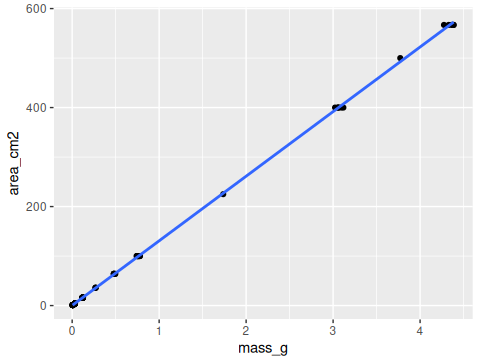
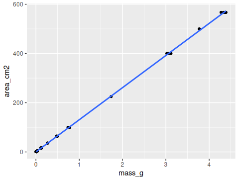
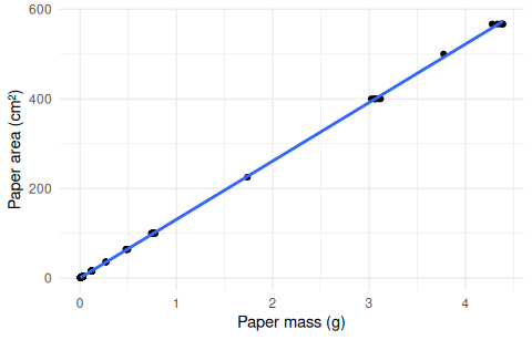
The shaded band = 95% confidence band for the mean predicted area at each mass value.

Key observation: the band is narrowest in the middle of the data range and widens at the extremes — predictions are most precise near \(\bar{X}\).

This is exactly Figure 17.2-1 from W&S (p. 549).

📖 W&S §17.2 p. 548–550

Check Assumptions — Residual Plot

Note

🔮 Predict first: If the line fits well, what should the residuals-vs-fitted plot look like — a random flat cloud, a curve, or a funnel? Predict, then look.

# mutate() adds new columns to the data frame ----------
# Here we add the model's fitted values and residuals
# so we can plot them — recall mutate() from Lecture 03!
paper_resid_df <- paper_df %>%
  mutate(
    fitted = fitted(paper_lm_model),
    residuals = residuals(paper_lm_model)
  )

# Residuals vs Fitted — checks linearity & equal variance
resid_plot <- paper_resid_df %>%
  ggplot(aes(x = fitted, y = residuals)) +
  geom_point(alpha = 0.5) +
  geom_hline(yintercept = 0, linetype = "dashed", color = "red") +
  labs(x = "Fitted Values (cm²)", y = "Residuals (cm²)") +
  theme_minimal()

resid_plot

What to look for:

✅ Good: random cloud of points centered at zero; constant spread across all fitted values
❌ Bad: - Curved pattern → linearity violated - Fan shape (funnel) → unequal variance
📖 W&S §17.5 p. 559 (Figure 17.5-4)

Tip

The residual plot is the most important diagnostic. Always check it before interpreting your results.

Check Assumptions — QQ Plot and Shapiro-Wilk

# QQ plot of residuals — checks normality assumption --
qq_resid_plot <- paper_resid_df %>%
  ggplot(aes(sample = residuals)) +
  stat_qq() +
  stat_qq_line(color = "red", linewidth = 0.8) +
  labs(
    title = "Normal QQ Plot of Residuals",
    x = "Theoretical Quantiles",
    y = "Sample Quantiles (residuals)"
  ) +
  theme_minimal()

qq_resid_plot

# Shapiro-Wilk test on residuals — NOT on raw data ---
shapiro.test(residuals(paper_lm_model))


    Shapiro-Wilk normality test

data:  residuals(paper_lm_model)
W = 0.67735, p-value = 9.425e-15

Remember:

The normality assumption is about residuals, not raw data
H₀ (Shapiro-Wilk): residuals are normally distributed
p > 0.05 → proceed with confidence intervals and p-values

📖 W&S §17.5 p. 559

🛑 Pause — Do Activity Parts 8–10 Now

Plot the calibration curve, then check the residual plot and the QQ/Shapiro test on the residuals. Predict each diagnostic before you run it.

🧩 Chunk 4 of 4 · Predict & Report

We will cover: turning a tracing mass into a predicted area, predict() with confidence vs prediction intervals, and writing the results paragraph.

Tip

🖐 After this chunk: Activity Parts 11–12 (predict leaf area; write the results paragraph).

Predict Leaf Area from Tracing Mass

Note

🔮 Predict first: The sunny tracing weighs 0.092 g, the shady 0.138 g. Before running — which predicts the larger area, and does that match “shady leaves are bigger”?

# Plug tracing masses into the calibration line -------
# Suppose sunny leaf tracing weighs 0.092 g
# and shady leaf tracing weighs 0.138 g

mass_sunny <- 0.092
mass_shady <- 0.138

area_sunny <- b_slope * mass_sunny + a_intercept
area_shady <- b_slope * mass_shady + a_intercept

cat("Sunny tracing mass:", mass_sunny, "g\n")

Sunny tracing mass: 0.092 g

cat("Predicted area:    ", round(area_sunny, 2), "cm²\n\n")

Predicted area:     12.29 cm²

cat("Shady tracing mass:", mass_shady, "g\n")

Shady tracing mass: 0.138 g

cat("Predicted area:    ", round(area_shady, 2), "cm²\n")

Predicted area:     18.29 cm²

The equation in action:

\[\widehat{\text{area}} = 130.5 \times \text{mass} + 0.28\]

For a sunny tracing at 0.092 g:

\(130.5 \times 0.092 + 0.28 = 12.3\) cm²

For a shady tracing at 0.138 g:

\(130.5 \times 0.138 + 0.28 = 18.3\) cm²

This matches our observation from Lecture 03 — shady leaves are larger!

Live Demo — Watch It Break (on purpose)

predict() needs the exact predictor column name. I’ll get it wrong:

# The column is mass_g, but I typed mass
new <- tibble(mass = 0.092)
predict(paper_lm_model, newdata = new)

R errors:

Error in eval(predvars, data, env) :
  object 'mass_g' not found

The fix — match the model’s variable name exactly:

new <- tibble(mass_g = 0.092)
predict(paper_lm_model, newdata = new)

Tip

✅ Why show a broken run?

predict() looks for the same column names the model was built on. “object ‘mass_g’ not found” means your newdata is missing that column — almost always a typo. This is the #1 predict() mistake.

Using `predict()` — with Prediction Intervals

# predict() gives uncertainty around predictions ------
new_masses <- tibble(mass_g = c(0.092, 0.138))

# Confidence interval: for the MEAN area at this mass
predict(paper_lm_model, newdata = new_masses, interval = "confidence") %>%
  round(3)

     fit    lwr    upr
1 12.287 11.940 12.635
2 18.291 17.948 18.634

# Prediction interval: for a SINGLE new observation
predict(paper_lm_model, newdata = new_masses, interval = "prediction") %>%
  round(3)

     fit    lwr    upr
1 12.287  8.777 15.798
2 18.291 14.782 21.801

Two types of interval (W&S §17.2 p. 549):

Type	Predicts	Width
Confidence	mean area for all leaves this mass	narrower
Prediction	area of one specific leaf	wider

For predicting a single leaf, use the prediction interval — it captures individual-to-individual variation within the same mass class.

📖 W&S §17.2 pp. 548–550

How to Report Regression Results

# Pull reporting values from the model ----------------
f_stat <- summary(paper_lm_model)$fstatistic
f_val <- round(f_stat[1], 1)
df1 <- f_stat[2]
df2 <- f_stat[3]
p_val <- pf(f_stat[1], df1, df2, lower.tail = FALSE)

cat("--- Results paragraph ---\n")

--- Results paragraph ---

cat("Paper mass was a strong predictor of paper area\n")

Paper mass was a strong predictor of paper area

cat("(linear regression: F(", df1, ",", df2, ") =", f_val, ",\n")

(linear regression: F( 1 , 116 ) = 784932.9 ,

cat("p <", signif(p_val, 1), ", R² =", round(r2_val, 4), ").\n")

p < 5e-224 , R² = 0.9999 ).

cat("The calibration equation is:\n")

The calibration equation is:

cat("  area =", round(b_slope, 2), "× mass +", round(a_intercept, 3), "cm²\n")

  area = 130.52 × mass + 0.279 cm²

cat(
  "(slope 95% CI:",
  round(confint(paper_lm_model)[2, 1], 2),
  "to",
  round(confint(paper_lm_model)[2, 2], 2),
  "cm²/g)\n"
)

(slope 95% CI: 130.23 to 130.82 cm²/g)

Standard report format:

“Paper area was accurately predicted from paper mass (linear regression: F(df₁, df₂) = F, p < 0.001, R² = 0.9999). The regression equation was area = 130.5 × mass + 0.28 (slope 95% CI: X to Y cm²/g).”

Always include: - F-statistic and both df - p-value (never “p = 0.000” — write “p < 0.001”) - R² - The actual equation - 95% CI for the slope

📖 W&S §17.3 p. 553

🛑 Pause — Do Activity Parts 11–12 Now

Predict leaf area from tracing mass, compare confidence vs prediction intervals, and write your results paragraph. Predict the numbers before they print.

What We Learned Today

Concepts:

Regression predicts Y from X using a straight line equation
Equation: \(\hat{Y} = a + bX\) — slope b, intercept a
Least squares — minimizes sum of squared residuals
R² — fraction of Y variation explained by X
Four assumptions — linearity, independence, equal variance, normality of residuals
Two prediction types — confidence vs. prediction intervals

R skills:

lm(Y ~ X, data) — fits the model
summary() — extracts slope, intercept, R², p-values
coef(), fitted(), residuals() — pull model components
mutate() with fitted() and residuals() — add model output to a data frame
predict(model, newdata, interval = "prediction") — predictions with uncertainty
geom_smooth(method = "lm", se = TRUE) — plot the line with CI band

Chapter references:

📖 W&S §17.1 — Linear regression
📖 W&S §17.2 — Confidence in predictions
📖 W&S §17.3 — Testing slope hypotheses
📖 W&S §17.4 — R²
📖 W&S §17.5 — Assumptions

Up next — Lecture 07:

Downloading real climate data straight into R with GSODR
Summarizing daily data to reveal long-term trends
Reusing lm() to estimate a rate of change over time

Lecture 06 — Linear Regression

Where we left off (Lecture 05)

Goals for Today

How to Use These Slides — Predict · Type · Run

🧩 Chunk 1 of 4 · What Regression Is

Our Calibration Idea

What Is Linear Regression?

The Regression Equation

Residuals and Least Squares

R² — How Much Does X Explain?

Assumptions of Regression

🛑 Pause — Do Activity Parts 1–3 Now

🧩 Chunk 2 of 4 · Fit the Model & Read It

Load Libraries and Data

Inspect the Data

First Plot — Scatter

Fit the Model with lm() - Linear Model

Reading the summary() Output

The Calibration Equation and R²

🛑 Pause — Do Activity Parts 4–7 Now

🧩 Chunk 3 of 4 · Visualize & Check Assumptions

Plot the Calibration Curve

Check Assumptions — Residual Plot

Check Assumptions — QQ Plot and Shapiro-Wilk

🛑 Pause — Do Activity Parts 8–10 Now

🧩 Chunk 4 of 4 · Predict & Report

Predict Leaf Area from Tracing Mass

Live Demo — Watch It Break (on purpose)

Using predict() — with Prediction Intervals

How to Report Regression Results

🛑 Pause — Do Activity Parts 11–12 Now

What We Learned Today

Fit the Model with `lm() - Linear Model`

Reading the `summary()` Output

Using `predict()` — with Prediction Intervals