Lecture 06 — Summary Statistics

Mean, median, spread, and describing groups the tidy way

Bill Perry

2026-10-01

Where we left off (Lecture 05 — Wrangling)

• filter(), select(), mutate(), arrange() — the core wrangling verbs
• Chaining verbs into one pipeline with %>%
• Our leaf data: leaf_df — shade, mass_g, petiole_mm, thickness_mm, paper_mass_g

Note

✅ Key idea from Lecture 05

You can already reshape the data into exactly the rows and columns you need. Today we learn to describe what’s in it — one number at a time, then all at once.

Our Scientific Question

Biological prediction: Leaves on the shady side of a tree will be larger and heavier to capture more of the limited light.

	Hypothesis
H₀ — null	No difference in leaf size between sunny and shady sides
Hₐ — alternate	Leaf size differs between sunny and shady sides

Plan for this unit:

1. Today — describe the data
2. Lecture 09 — formally test the hypotheses with a t-test

Statistics helps us decide which hypothesis is better supported by the data.

References:

• 📖 Whitlock & Schluter, Ch. 3 — Describing Data
• 📖 Whitlock & Schluter, Ch. 4 — Estimating with Uncertainty
• 📖 R4DS Ch 13 — Numbers
• 📖 R4DS Ch 18 — Missing Values

Both W&S PDFs are in the course readings/ folder.

How to Use These Slides — Predict · Type · Run

This lecture runs in two chunks. After each chunk you switch to the activity and type the code yourself into your R script.

For every code block, do three things:

1. Predict — before it runs, say what you think the output will be
2. Type it out by hand — do not copy-paste
3. Run it and compare to your prediction

Note

✅ Why bother?

• A single mean or SD looks obvious once it’s on the slide — predicting it first is what tells you whether you actually understand where the number comes from.
• Typing sum(!is.na(x)) yourself, instead of pasting it, is what makes you notice why it’s there instead of length(x).

Load Libraries and Data

# Load all packages at the top of every script ----------
library(readxl) # reading Excel files
library(tidyverse) # data wrangling + ggplot2
library(janitor) # clean_names()
library(skimr) # fast descriptive summaries

# Read the leaf data from the data folder ---------------
leaf_df <-
  read_excel("data/2026_09_03_data_sci_leaf_area.xlsx") %>%
  clean_names()

Note

Install once — load every session

• Run in the Console one time only: install.packages("skimr")
• Then every session: library(skimr) activates it.

Tip

📂 Activity skeleton: 06_summary_stats_skeleton.R has this loading step, plus both source() lines below, already done for you.

🧩 Chunk 1 of 2 · Build and Use summary_stats()

We will cover: finding NAs in real data, counting correctly with sum(!is.na()), writing the summary by hand with group_by() + summarize(), and only then packaging it into a reusable summary_stats() helper.

What Is the Mean?

\[\bar{x} = \frac{\sum_{i=1}^{n} x_i}{n}\]

• Add up all values, divide by n
• The balance point of the distribution
• Sensitive to outliers — one very large value pulls the mean up

Example:

Values: 5, 6, 7, 8, 50 → mean = 15.2

Is 15.2 a fair summary? Not really — the outlier dominates!

Why it matters:

• The most commonly reported statistic
• Used in every t-test, ANOVA, and regression
• Always pair it with a measure of spread (SD or SE)

📖 Whitlock & Schluter, Ch. 3 — Describing Data; R4DS §13 — Numbers

What Is the Median?

The middle value when data are sorted

Sorted data	Median
5, 6, 7, 8, 50	7
5, 6, 7, 8, 50, 51	(7 + 8) / 2 = 7.5

• Not pulled by outliers → robust

• If mean ≫ median → right-skewed
• If mean ≈ median → roughly symmetric
• skim() reports the median for us later today — no code to type by hand

Counting Correctly — sum(!is.na())

# length() counts ALL positions — including NAs -------
x <- c(4, 3, NA, 7, NA) # a vector with missing values

length(x) # returns 5 — but 2 are NA!

[1] 5

sum(!is.na(x)) # sum() counts the TRUEs = real values

[1] 3

• length(x) counts all positions — including NA
• is.na(x) → TRUE for each NA; !is.na(x) flips it to TRUE for real values
• sum(!is.na(x)) counts those TRUEs → the correct n
• This is a silent error — R never warns you
• Our leaf data has real NAs too: not every leaf got a paper_mass_g measurement

📖 R4DS §18 — Missing Values

Tip

Best practice: always use sum(!is.na(x)) when you need n — even when you think there are no NAs.

Finding the NAs in Real Data

# Which rows are MISSING a paper_mass_g value? ---------
leaf_df %>%
  filter(is.na(paper_mass_g))

# A tibble: 13 × 8
   twig_id leaf_id teams     shade mass_g petiole_mm thickness_mm
   <chr>   <chr>   <chr>     <chr>  <dbl>      <dbl>        <dbl>
 1 twig_2  l09     fighting… shady  0.920      0.383        NA   
 2 <NA>    1       Oscar_Ka… shady  0.454     53.6           0.36
 3 <NA>    2       Oscar_Ka… shady  0.371     26.3           0.43
 4 <NA>    3       Oscar_Ka… shady  0.351     57.8           0.48
 5 <NA>    4       Oscar_Ka… shady  0.453     51.0           0.41
 6 <NA>    5       Oscar_Ka… shady  0.344     37.0           0.25
 7 <NA>    6       Oscar_Ka… shady  0.426     66.3           0.5 
 8 <NA>    1       Oscar_Ka… sunny  0.357     48.7           0.41
 9 <NA>    2       Oscar_Ka… sunny  0.348     44.8           0.39
10 <NA>    3       Oscar_Ka… sunny  0.511     63.4           0.53
11 <NA>    4       Oscar_Ka… sunny  0.230     35.7           0.36
12 <NA>    5       Oscar_Ka… sunny  0.304     51.3           0.43
13 <NA>    6       Oscar_Ka… sunny  0.282     46.9           0.4 
# ℹ 1 more variable: paper_mass_g <dbl>

# Flip it with ! — keep only the rows that HAVE a value
leaf_df %>%
  filter(!is.na(paper_mass_g))

# A tibble: 40 × 8
   twig_id leaf_id teams shade mass_g petiole_mm thickness_mm
   <chr>   <chr>   <chr> <chr>  <dbl>      <dbl>        <dbl>
 1 <NA>    <NA>    12345 sunny   0.4          79         0.15
 2 <NA>    <NA>    12345 sunny   0.48         63         0.14
 3 <NA>    <NA>    12345 sunny   0.34         68         0.14
 4 <NA>    <NA>    12345 sunny   0.65         35         0.15
 5 <NA>    <NA>    12345 sunny   0.27         34         0.11
 6 <NA>    <NA>    12345 sunny   0.43         40         0.16
 7 <NA>    <NA>    12345 shady   0.39         40         0.14
 8 <NA>    <NA>    12345 shady   0.45         65         0.15
 9 <NA>    <NA>    12345 shady   0.6          68         0.12
10 <NA>    <NA>    12345 shady   0.57         73         0.14
# ℹ 30 more rows
# ℹ 1 more variable: paper_mass_g <dbl>

• filter(is.na(paper_mass_g)) shows you the problem — every row where the measurement is missing
• filter(!is.na(paper_mass_g)) keeps the rows with real values — the same ! idea as sum(!is.na())
• Look at the row counts: the two tables together add back up to nrow(leaf_df)
• Do this before any statistics — you cannot trust a mean until you know what is missing

📖 R4DS §18 — Missing Values

What Is Variance?

\[s^2 = \frac{\sum_{i=1}^{n}(x_i - \bar{x})^2}{n - 1}\]

1. For each value, compute distance from mean: \((x_i - \bar{x})\)
2. Square those distances → all positive
3. Sum them up, divide by \(n - 1\), not \(n\)

Larger variance = more spread = more uncertainty

Note

Why \(n - 1\), not \(n\)?

Estimating \(\bar{x}\) already used up one piece of information, leaving only \(n - 1\) degrees of freedom to estimate spread. Dividing by \(n - 1\) instead of \(n\) corrects for that, so \(s^2\) comes out an unbiased estimate of the population variance.

What Is Standard Deviation?

\[s = \sqrt{s^2} = \sqrt{\frac{\sum(x_i - \bar{x})^2}{n-1}}\]

• The square root of variance → back in original units (g) ✓
• Reports how spread out individual data points are
• Variance is in squared units (g²) — hard to interpret. That is why we use SD.

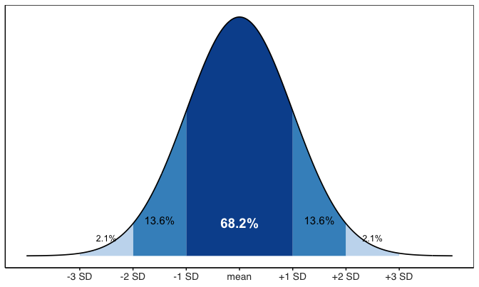
For a normal distribution, each band is a fixed percent of the data — no matter what the mean or SD actually are.

What Is Standard Error?

\[SE = \frac{s}{\sqrt{n}}\]

• Measures how precisely we know the mean
• Not the spread of raw data — the uncertainty of the mean itself
• Gets smaller as n increases → more data = more precise estimate

	Describes
SD	spread of individual data points
SE	precision of the sample mean

We report SE when making claims about group means.

📖 Whitlock & Schluter, Ch. 4 — Estimating with Uncertainty

Do It By Hand First — One Group

# Every statistic, written out, for the sunny leaves ----
leaf_df %>%
  filter(shade == "sunny") %>%
  summarize(
    mean     = mean(mass_g, na.rm = TRUE),
    variance = var(mass_g, na.rm = TRUE),
    sd       = sd(mass_g, na.rm = TRUE),
    n        = sum(!is.na(mass_g)),
    se       = sd / sqrt(n)
  )

# A tibble: 1 × 5
   mean variance    sd     n     se
  <dbl>    <dbl> <dbl> <int>  <dbl>
1 0.505   0.0442 0.210    25 0.0421

• summarize() collapses many rows down to one row of statistics
• Every function gets na.rm = TRUE — otherwise one NA makes the whole answer NA
• n = sum(!is.na(mass_g)) — the correct count, not n()
• se = sd / sqrt(n) — you can reuse sd and n later in the same summarize(), because they are already columns by then
• The result is a data frame, so it pipes onward into ggplot() or write_csv()

Do It By Hand — Every Group at Once

Note

🔮 Predict first: How many rows will this return? (Hint: how many values does shade take?)

# group_by() splits the data; summarize() runs per group
leaf_df %>%
  group_by(shade) %>%
  summarize(
    mean     = mean(mass_g, na.rm = TRUE),
    variance = var(mass_g, na.rm = TRUE),
    sd       = sd(mass_g, na.rm = TRUE),
    n        = sum(!is.na(mass_g)),
    se       = sd / sqrt(n)
  )

# A tibble: 2 × 6
  shade  mean variance    sd     n     se
  <chr> <dbl>    <dbl> <dbl> <int>  <dbl>
1 shady 0.523   0.0219 0.148    28 0.0280
2 sunny 0.505   0.0442 0.210    25 0.0421

• Exactly the same summarize() — the only new line is group_by(shade)
• One row per group instead of one row overall
• This is the workhorse pattern for the rest of the course

Note

✅ Key idea

Running this once for sunny and again for shady is exactly the repetition group_by() exists to remove.

Now Package It — summary_stats()

summary_stats <- function(data, variable) {
  data %>%
    summarize(
      n        = sum(!is.na({{ variable }})),
      mean     = mean({{ variable }}, na.rm = TRUE),
      variance = var({{ variable }}, na.rm = TRUE),
      sd       = sd({{ variable }}, na.rm = TRUE),
      se       = sd / sqrt(n),
      ci_lower = mean - qt(0.975, df = n - 1) * se,
      ci_upper = mean + qt(0.975, df = n - 1) * se,
      .groups  = "drop"
    )
}

• It is the same summarize() you just wrote by hand — wrapped in function() so you type it once, not once per variable
• Plus a 95% confidence interval for the mean, for free
• { variable } lets you pass a bare column name in, like mass_g
• Works on one group or, if the data are already group_by()-ed, every group at once
• Source: themes/summary_stats_function.R — same themes/ folder as your ggplot theme file

# source() loads summary_stats() from another .R file --
source("themes/summary_stats_function.R")

One Group at a Time — filter() + summary_stats()

# Filter to one side, then hand it straight to the function
leaf_df %>%
  filter(shade == "sunny") %>%
  summary_stats(mass_g)

# A tibble: 1 × 7
      n  mean variance    sd     se ci_lower ci_upper
  <int> <dbl>    <dbl> <dbl>  <dbl>    <dbl>    <dbl>
1    25 0.505   0.0442 0.210 0.0421    0.418    0.592

• filter(shade == "sunny") — keeps only sunny rows
• Pipe the filtered data straight into summary_stats(mass_g) — no pull(), no vector, no hand-written math
• Swap "sunny" for "shady" to get the other side

📖 R4DS §3 — Data Transformation

🛑 Pause — Do Activity Parts 1–3 Now

🛑 Do Activity Parts 1–3 now

Load the data, find the NAs, write the summary by hand with group_by() + summarize(), then source summary_stats() and use it on one group. Predict each output, type it, then run it.

🧩 Chunk 2 of 2 · Every Group, Every Column, Fast

We will cover: group_by() + summary_stats() for every group at once, fast overviews with skimr, and — if time allows — across() for many columns at once.

🛑 After this chunk: Activity Parts 4–6.

Stats the Tidy Way — group_by() + summary_stats()

Note

🔮 Predict first: How many rows will this return? (Hint: how many values does shade take?) Predict the number before you run it.

# Group first, then call the SAME function -------------
stats_df <- leaf_df %>%
  group_by(shade) %>%
  summary_stats(mass_g)

stats_df

# A tibble: 2 × 8
  shade     n  mean variance    sd     se ci_lower ci_upper
  <chr> <int> <dbl>    <dbl> <dbl>  <dbl>    <dbl>    <dbl>
1 shady    28 0.523   0.0219 0.148 0.0280    0.466    0.580
2 sunny    25 0.505   0.0442 0.210 0.0421    0.418    0.592

• group_by(shade) splits the data by the shade column
• summary_stats() doesn’t change at all — it runs once per group
• You get both groups, every statistic, in one clean table

📖 R4DS §3.5 — summarize()

Multiple Variables at Once

# summary_stats() handles ONE variable, so for several
# measurements at once we still write summarize() directly
size_stats_df <- leaf_df %>%
  group_by(shade) %>%
  summarize(
    n          = sum(!is.na(mass_g)),
    mean_mass  = mean(mass_g, na.rm = TRUE),
    mean_pet   = mean(petiole_mm, na.rm = TRUE),
    mean_thick = mean(thickness_mm, na.rm = TRUE)
  )

size_stats_df

# A tibble: 2 × 5
  shade     n mean_mass mean_pet mean_thick
  <chr> <int>     <dbl>    <dbl>      <dbl>
1 shady    28     0.523     56.7      0.356
2 sunny    25     0.505     54.4      0.290

Do the numbers support our hypothesis?

• Shady heavier? → check mean_mass
• Shady leaves thicker? → check mean_thick
• Shady petioles longer? → check mean_pet

Fast Summaries with skimr

# skim() grouped by shade — mass only -------------------
leaf_df %>%
  select(shade, mass_g) %>%
  group_by(shade) %>%
  skim()

Data summary

Name	Piped data
Number of rows	53
Number of columns	2
_______________________
Column type frequency:
numeric	1
________________________
Group variables	shade

Variable type: numeric

skim_variable	shade	n_missing	complete_rate	mean	sd	p0	p25	p50	p75	p100	hist
mass_g	shady	0	1	0.52	0.15	0.34	0.42	0.52	0.59	0.92	▇▅▃▁▁
mass_g	sunny	0	1	0.51	0.21	0.19	0.35	0.48	0.65	1.08	▇▇▆▃▁

skim() is your fastest first look — n_missing, mean, SD, percentiles, and a mini histogram, per group, in one line.

The Fast Way — across()

# Apply the SAME function to every numeric column -----
mean_all_df <- leaf_df %>%
  group_by(shade) %>%
  summarize(
    across(
      c(mass_g, petiole_mm, thickness_mm),
      ~ mean(.x, na.rm = TRUE)
    )
  )

mean_all_df

# A tibble: 2 × 4
  shade mass_g petiole_mm thickness_mm
  <chr>  <dbl>      <dbl>        <dbl>
1 shady  0.523       56.7        0.356
2 sunny  0.505       54.4        0.290

• across(columns, function) applies one function to many columns at once
• .x is a stand-in for “whichever column we’re on right now”
• Same idea as mean_mass/mean_thick/mean_pet above — just without typing each one out

Tip

Once you have more than 3–4 measurement columns, across() saves real typing — and real typos.

→ ACTIVITY 6 starts now

🛑 Go to Activity 6 — Summary Statistics

Close the slides. Finish Activity Parts 4–6, then Part 7 (review and checkpoint) on your own.

What We Learned Today

• Statistics concepts:
  • Mean — balance point; sensitive to outliers
  • Median — middle value; robust
  • Variance / SD — spread of individual data; \(n-1\) makes \(s^2\) unbiased
  • SE — precision of the sample mean
• R skills:
  • filter(is.na()) / filter(!is.na()) — see the missing data before you summarize
  • sum(!is.na()) — the right way to count n
  • group_by() + summarize() by hand — mean, variance, sd, n, se
  • The same code packaged as a reusable summary_stats() function, sourced from themes/
  • group_by() — run the same summary on every group at once
  • skim() — instant full dataset overview
  • across() — one function, many columns

References:

• 📖 Whitlock & Schluter, Ch. 3 — Describing Data
• 📖 Whitlock & Schluter, Ch. 4 — Estimating with Uncertainty
• 📖 R4DS §13 — Numbers
• 📖 R4DS §18 — Missing Values

Both W&S PDFs are in the course readings/ folder.

Up next — Lecture 07, Quarto:

• Writing reproducible reports
• Mixing prose, code, and results in one document