The two-sample Welch’s t-test from assumptions to results
2026-07-05
filter(), select(), mutate(), arrange() as the core tidyverse verbsgroup_by() + summarize()sum(!is.na()) is the safe way to count nskimr — fast full-dataset overview in one linestat_summary()Note
✅ Key idea from Lecture 03
We described the pattern in our data. Today we formally test whether that pattern is statistically significant.
t.test() outputTip
🖐 Try it yourself
By the end you will run and interpret a complete t-test on our leaf data.
Tools added today:
car — Levene’s variance testReferences:
Today’s naming:
_model_plotBiological prediction:
Shady-side leaves will be larger and heavier — they need more surface area to capture the limited light filtering through the canopy.
| Formal statement | |
|---|---|
| H₀ — null | \(\mu_{shady} = \mu_{sunny}\) — no difference in mean leaf weight |
| Hₐ — alternate | \(\mu_{shady} \neq \mu_{sunny}\) — mean leaf weight differs by side |
We use a two-tailed test — we will detect a difference in either direction.
Why two-tailed?
α = 0.05 — our threshold for rejecting H₀
This lecture runs in four short chunks. After each chunk you switch to the activity worksheet and type the code yourself.
For every code block, do three things:
Note
✅ Why bother? (the evidence)
Note
car is the Companion to Applied Regression package. It contains leveneTest(), which we use to check whether our two groups have similar variance.
Install once: install.packages("car")
Note
🔮 Predict first: The two group means differ by about 4 g. With only 10 leaves per side — commit now to a yes/no: is that gap big enough to be statistically significant? You’ll find out in Chunk 3.
# A tibble: 2 × 5
side n mean_wt sd_wt se_wt
<chr> <int> <dbl> <dbl> <dbl>
1 shady 10 7.8 1.03 0.33
2 sunny 10 3.8 0.79 0.25
We will cover: why comparing means isn’t enough, what a two-sample t-test is, why we default to Welch’s, and the formula in action.
Tip
🖐 After this chunk: Activity Parts 1–3 (load data, state hypotheses, recap the descriptive stats).
# Remind ourselves what the data look like ---------------
recap_plot <- tree_df %>%
ggplot(aes(x = side, y = weight_g, color = side)) +
geom_point(
position = position_jitter(width = 0.15, seed = 42),
alpha = 0.5,
size = 2
) +
stat_summary(fun = mean, geom = "point", size = 4) +
stat_summary(
fun.data = mean_se,
geom = "errorbar",
width = 0.15,
linewidth = 0.9
) +
labs(x = "Side", y = "Leaf Weight (g)") +
theme_minimal() +
theme(legend.position = "none")
recap_plot
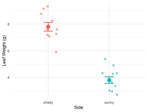
The means look different — but:
A p-value tells us:
“If H₀ were true, how often would we see a gap this large just by chance?”
Small p → the gap is unlikely to be chance.
A two-sample t-test compares the means of two independent groups.
It asks: Could both groups plausibly be drawn from populations with the same mean?
The t-statistic is:
\[t = \frac{\bar{x}_1 - \bar{x}_2}{\text{SE}_{\text{diff}}}\]
Large |t| → the difference is large relative to the noise → small p-value
| Component | Our context |
|---|---|
| Group 1 | Shady leaves |
| Group 2 | Sunny leaves |
| Measurement | weight_g |
| H₀ | \(\mu_{shady} = \mu_{sunny}\) |
| Hₐ | \(\mu_{shady} \neq \mu_{sunny}\) |
Standard t-test — pools the two variances into one estimate. Requires both groups to have the same population variance.
Welch’s t-test — uses each group’s variance separately. Does not require equal variance.
\[t_W = \frac{\bar{x}_1 - \bar{x}_2}{\sqrt{\dfrac{s_1^2}{n_1} + \dfrac{s_2^2}{n_2}}}\]
The denominator is the true SE of the difference — no pooling.
Why always use Welch’s?
Tip
Best practice: use Welch’s as your default for all two-group comparisons.
In R: var.equal = FALSE
Note
🔮 Predict first: t = difference ÷ SE-of-the-difference, and the difference is 4 g. Do you expect |t| to land nearer 1, 5, or 10? Predict before the numbers appear.
# Pull stats and compute t by hand ----------------------
stats_df <- tree_df %>%
group_by(side) %>%
summarize(
n = sum(!is.na(weight_g)),
m = mean(weight_g, na.rm = TRUE),
s = sd(weight_g, na.rm = TRUE)
)
m_sha <- stats_df$m[stats_df$side == "shady"]
m_sun <- stats_df$m[stats_df$side == "sunny"]
s_sha <- stats_df$s[stats_df$side == "shady"]
s_sun <- stats_df$s[stats_df$side == "sunny"]
n_sha <- stats_df$n[stats_df$side == "shady"]
n_sun <- stats_df$n[stats_df$side == "sunny"]
se_diff <- sqrt((s_sha^2 / n_sha) + (s_sun^2 / n_sun))
t_manual <- (m_sha - m_sun) / se_diff
cat("Difference in means:", round(m_sha - m_sun, 2), "g\n")Difference in means: 4 g
SE of difference: 0.411
t-statistic: 9.733
Step by step:
The observed difference is ~10 standard errors above zero — very far from what we’d expect if H₀ were true.
Load the data, write your hypotheses before looking at any results, and recompute the group means / SD / SE. Predict each output, type it, run it.
We will cover: the five-step framework, stating H₀ / Hₐ, and checking normality (histogram, QQ, Shapiro-Wilk) and equal variance (Levene’s).
Tip
🖐 After this chunk: Activity Parts 4–7 (histogram, QQ, Shapiro, Levene).
We will always follow this sequence:
| Step | Action |
|---|---|
| 1 | State H₀ and Hₐ |
| 2 | Check normality — histogram/box plot |
| 3 | Check normality — QQ plot + Shapiro-Wilk |
| 4 | Check variance — Levene’s test |
| 5 | Run the test; interpret and report |
Important
Check assumptions BEFORE running the test.
If your data seriously violate assumptions, the p-value from the t-test is unreliable.
With n = 10 per group, our main concern is gross non-normality. The t-test is quite robust to mild departures.
Null hypothesis:
\[H_0: \mu_{shady} = \mu_{sunny}\]
Shady and sunny leaves have the same mean weight in the population.
Alternate hypothesis (two-tailed):
\[H_A: \mu_{shady} \neq \mu_{sunny}\]
The mean leaf weights differ between sides — in either direction.
Significance level: α = 0.05
We will reject H₀ if p < 0.05.
Why state hypotheses first?
Our commitment: two-tailed, α = 0.05, before running any test.
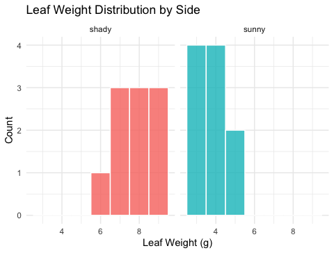
# Histogram per group to visually check normality -------
hist_norm_plot <- tree_df %>%
ggplot(aes(x = weight_g, fill = side)) +
geom_histogram(binwidth = 1, color = "white", alpha = 0.8) +
facet_wrap(~side, ncol = 2) +
labs(
title = "Leaf Weight Distribution by Side",
x = "Leaf Weight (g)",
y = "Count"
) +
theme_minimal() +
theme(legend.position = "none")
hist_norm_plot
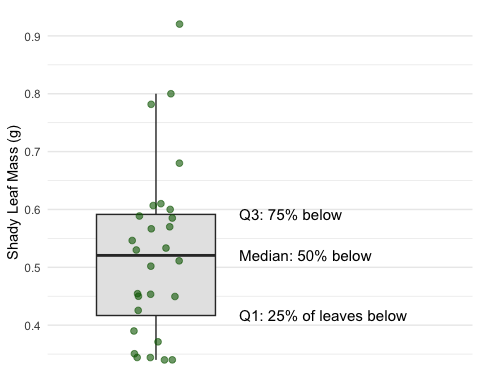
What to look for:
With n = 10 per group, histograms look lumpy — that is normal for small samples.
Histograms are a visual check only. We also use QQ plots and Shapiro-Wilk.
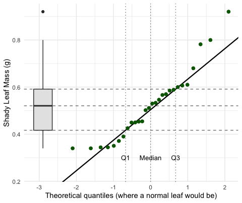
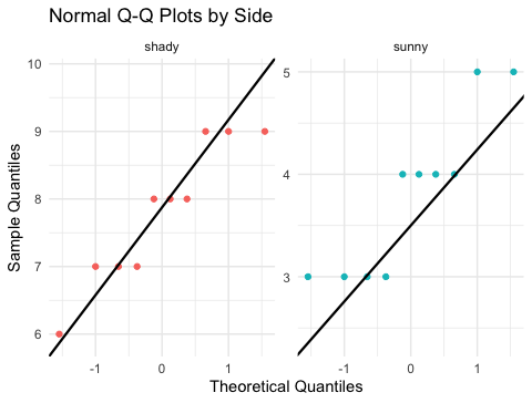
# Q-Q plot — points should fall along the diagonal line --
qq_norm_plot <- tree_df %>%
ggplot(aes(sample = weight_g, color = side)) +
stat_qq() +
stat_qq_line(color = "black", linewidth = 0.8) +
facet_wrap(~side, scales = "free") +
labs(
title = "Normal Q-Q Plots by Side",
x = "Theoretical Quantiles",
y = "Sample Quantiles"
) +
theme_minimal() +
theme(legend.position = "none")
qq_norm_plot
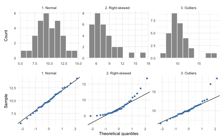
How to read a QQ plot:
If points follow the line roughly, we are comfortable proceeding with the t-test.
Note
🔮 Predict first: Shapiro-Wilk’s H₀ is “the data are normal.” From the histogram and QQ plot you just saw, predict for each side: will p be above or below 0.05?
Shapiro-Wilk normality test
data: .
W = 0.8197, p-value = 0.02513
Shapiro-Wilk H₀: the data are normally distributed.
Important
Small-sample caution:
With n = 10, this test has low power — it rarely detects non-normality even when present. The QQ plot is equally important.
Levene’s test H₀: the two groups have equal variance.
Our response regardless of the result:
We will use Welch’s t-test (var.equal = FALSE).
Welch’s is valid whether or not the variances are equal. We run Levene’s to understand our data, not to choose our test.
Suppose I forgot library(car) and run Levene’s:
R stops with:
Error in leveneTest(weight_g ~ side, data = tree_df) :
could not find function "leveneTest"
The fix — load the package that contains the function:
Tip
✅ Why show a broken run?
“could not find function” almost always means a missing library() — not a typo. Watching me diagnose it here means you’ll fix it in seconds when it happens to you.
Check every assumption before you test: histogram, QQ plot, Shapiro-Wilk, and Levene’s. Predict each p-value before you run it.
We will cover: running Welch’s t.test(), reading every line of the output, and making a formal reject / fail-to-reject decision.
Tip
🖐 After this chunk: Activity Parts 8–11 (run, decode, calculate t by hand, decide).
Note
🔮 Predict first: Write down a guess for the p-value before you run t.test() — above or below 0.05? Then see how close you were.
Welch Two Sample t-test
data: weight_g by side
t = 9.7333, df = 16.834, p-value = 2.514e-08
alternative hypothesis: true difference in means between group shady and group sunny is not equal to 0
95 percent confidence interval:
3.132297 4.867703
sample estimates:
mean in group shady mean in group sunny
7.8 3.8
Key arguments:
| argument | what it does |
|---|---|
weight_g ~ side |
compare weight_g between levels of side |
var.equal = FALSE |
use Welch’s correction |
alternative = "two.sided" |
two-tailed test |
The result is a model object. We decode each line of the output on the next slide.
t.test() Outputt-statistic : 9.733
df (Welch) : 16.83
p-value : 2.51e-08
95% CI : 3.13 to 4.87 g
Mean shady : 7.8 g
Mean sunny : 3.8 g
Line by line:
| output | meaning |
|---|---|
t |
our calculated t-statistic |
df |
Welch-Satterthwaite df (non-integer is normal!) |
p-value |
probability of this result if H₀ is true |
95% CI |
plausible range for the true difference in means |
mean of shady/sunny |
the two group means |
The 95% CI is the range we could expect to see if we repeated this study many times.
# State the decision formally --------------------------
# if/else: R checks the condition and runs one of two blocks
# We will learn these formally in the functions lecture
p_val <- leaf_ttest_model$p.value
alpha <- 0.05
if (p_val < alpha) {
cat("p =", signif(p_val, 3), "< α =", alpha, "\n")
cat("Decision: REJECT H₀\n")
cat("Conclusion: leaf weight differs between sides.\n")
} else {
cat("p =", signif(p_val, 3), ">= α =", alpha, "\n")
cat("Decision: FAIL TO REJECT H₀\n")
cat("Conclusion: insufficient evidence of a difference.\n")
}p = 2.51e-08 < α = 0.05
Decision: REJECT H₀
Conclusion: leaf weight differs between sides.
Important
What a small p-value means:
If H₀ were true (no real difference), we would get a t-statistic this large or larger less than p × 100% of the time just by chance.
We set α = 0.05 before the test. If p < α, we reject H₀.
What a small p-value does NOT mean:
Run the test, decode t / df / p / CI, reproduce t by hand, and state your decision in formal language. Predict the p-value first.
We will cover: embedding the test result in a boxplot and a mean ± SE plot, writing a scientific results sentence, and saving publication-quality figures.
Tip
🖐 After this chunk: Activity Parts 12–13 (plots and the results sentence).
# Final boxplot with all points -----------------------
leaf_box_04_plot <- tree_df %>%
ggplot(aes(x = side, y = weight_g, fill = side)) +
geom_boxplot(alpha = 0.5, outlier.shape = NA) +
geom_point(
position = position_jitter(width = 0.15, seed = 42),
alpha = 0.6,
size = 2.5
) +
labs(
title = "Leaf Weight by Tree Side",
subtitle = paste0(
"Welch's t-test: t = ",
round(leaf_ttest_model$statistic, 2),
", p = ",
signif(leaf_ttest_model$p.value, 2)
),
x = "Side of Tree",
y = "Leaf Weight (g)"
) +
theme_minimal() +
theme(legend.position = "none")
leaf_box_04_plot
Including the test result in the figure:
subtitle pulls t and p directly from the model objectTip
Embedding test statistics in the plot subtitle saves you from copying numbers by hand — and avoids typos in your report.
# Mean ± SE plot with individual points ---------------
leaf_mean_se_04_plot <- tree_df %>%
ggplot(aes(x = side, y = weight_g, color = side)) +
geom_point(
position = position_jitter(width = 0.15, seed = 42),
alpha = 0.35,
size = 2
) +
stat_summary(fun = mean, geom = "point", size = 4) +
stat_summary(
fun.data = mean_se,
geom = "errorbar",
width = 0.15,
linewidth = 0.9
) +
labs(
title = "Mean ± SE Leaf Weight by Tree Side",
subtitle = paste0(
"Welch's t: t(",
round(leaf_ttest_model$parameter, 1),
") = ",
round(leaf_ttest_model$statistic, 2),
", p < 0.001"
),
x = "Side of Tree",
y = "Leaf Weight (g)"
) +
theme_minimal() +
theme(legend.position = "none")
leaf_mean_se_04_plot
What the error bars tell you:
Rule of thumb:
If error bars overlap by less than half the bar length, the difference is likely significant at α = 0.05. The p-value from the t-test is the definitive answer.
--- Results sentence ---
Shady-side leaves were significantly heavier than
sunny-side leaves (Welch's t-test: t( 16.8 ) = 9.73 , p = 2.5e-08 ).
Mean ± SE: shady = 7.8 ± 0.33 g,
sunny = 3.8 ± 0.25 g.
Standard format:
“[Finding] (Welch’s t-test: t(df) = X.XX, p = X.XXX; mean ± SE: group1 = X.X ± X.X units, group2 = X.X ± X.X units).”
Always include:
Never report “p = 0.000” — write “p < 0.001” instead.
# Save both plots to the figures folder ----------------
ggsave(
"figures/leaf_weight_boxplot_ttest.png",
plot = leaf_box_04_plot,
width = 5,
height = 5,
units = "in",
dpi = 300
)
ggsave(
"figures/leaf_weight_mean_se_ttest.png",
plot = leaf_mean_se_04_plot,
width = 5,
height = 5,
units = "in",
dpi = 300
)Both plots are now in your figures/ folder with the test statistics embedded in the subtitle — ready for a lab report or paper.
Tip
dpi = 300 is publication quality. Use it for any figure that will appear in a paper, poster, or formal report.
Build both figures with the statistics embedded in the subtitle, then write your results sentence. Predict what the subtitle will say before you run it.
Concepts:
var.equal = FALSE as the safe defaultR skills:
library(car) + leveneTest(y ~ group, data) — variance checkfilter() %>% pull() %>% shapiro.test() — normality per groupt.test(y ~ group, data, var.equal = FALSE, alternative = "two.sided")model$statistic, model$p.value, model$conf.int — extract resultspaste0(...) in subtitle — embed test statistics in figuresReferences:
Up next — Lecture 05:
lm()