A Brief introduction to factors
Bill Perry
2019/10/26
Load Libraies
# Load Libraries ----
# this is done each time you run a script
library("readxl") # read in excel files
library("tidyverse") # dplyr and piping and ggplot etc
library("lubridate") # dates and times
library("scales") # scales on ggplot ases
library("skimr") # quick summary stats
library("janitor") # clean up excel imports
library("patchwork") # multipanel graphs
Read in files
# If you were typing in data this might be how it looks
# Read in wide dataframe ----
lakes.df <- read_csv("data/reduced_lake_long_genus_species.csv")
##
## ── Column specification ────────────────────────────────────────────────────────
## cols(
## permanent_id = col_double(),
## lake_name = col_character(),
## date = col_date(format = ""),
## group = col_character(),
## genus_species = col_character(),
## org_l = col_double(),
## year = col_double()
## )Factors are used to help convert a continuous or categorical variable into discrete categorical variables used in statistics
You will still see the variable as you normall would Lakes - Willis, Grass, Indian, South
What is really happening - they are alphabetized Indian, Grass, South Willis
and behind the scenes they are assigned a number 1 - n 1, 2, 3, 4
# Convert to factors -----
lakes.df <- lakes.df %>%
  mutate(lake_name = as.factor(lake_name))
# look at the levels
levels(lakes.df$lake_name)## [1] "Grass" "Indian" "South" "Willis"# What if we wanted them reordered to some particular order
lakes.df <- lakes.df %>%
mutate(
lake_name = fct_relevel(lake_name,
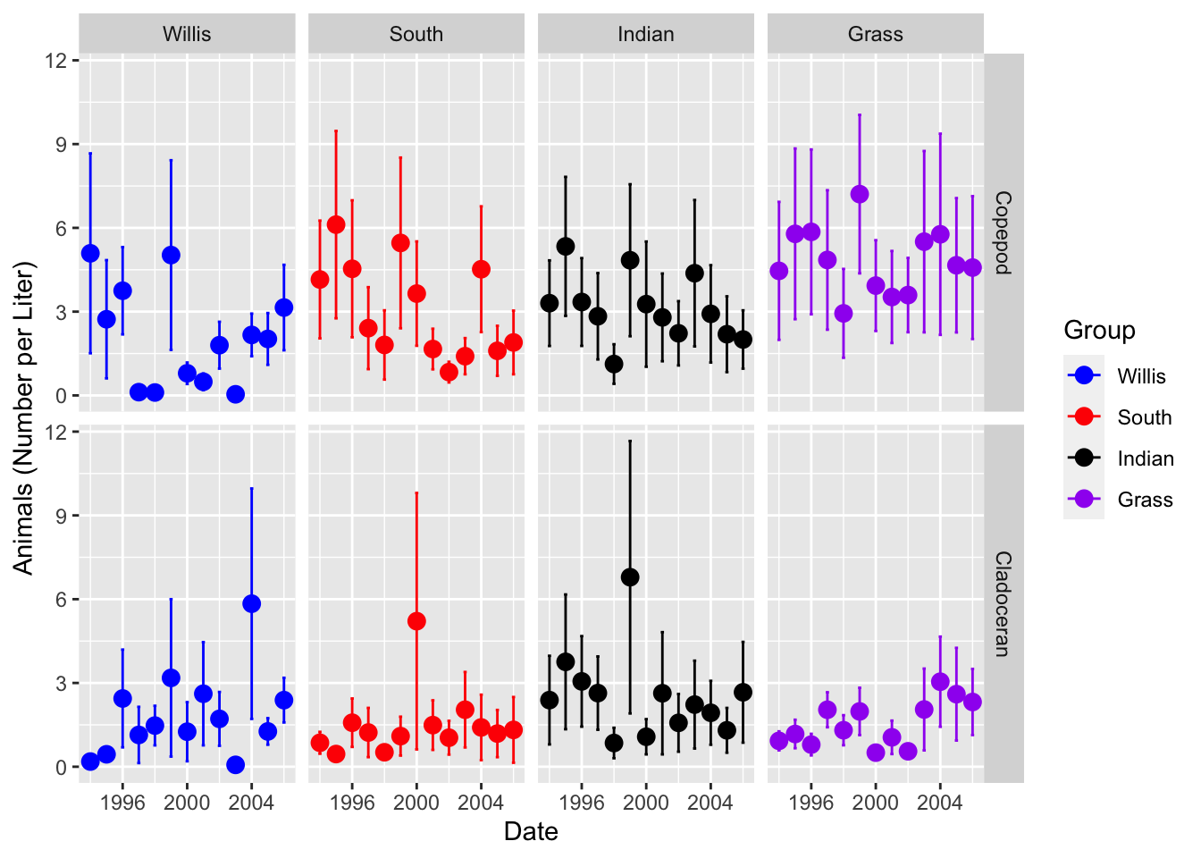
"Willis", "South", "Indian", "Grass"))# here is an example of where you might want it...
# we can offset the points so they dont overlap
lakes.df %>% ggplot(aes(year, color = lake_name)) +
stat_summary(aes(y = org_l),
fun.y = mean, na.rm = TRUE,
geom = "point",
size = 3,
position = position_dodge(0.2)) +
stat_summary(aes(y = org_l),
fun.data = mean_se, na.rm = TRUE,
geom = "errorbar",
width = 0.2,
position = position_dodge(0.2)) +
labs(x = "Date", y = "Animals (Number per Liter)") +
scale_color_manual(name = "Group",
values = c("blue", "red", "black", "purple"),
labels = c("Willis", "South", "Indian", "Grass")) +
facet_grid(group ~ lake_name)## Warning: `fun.y` is deprecated. Use `fun` instead.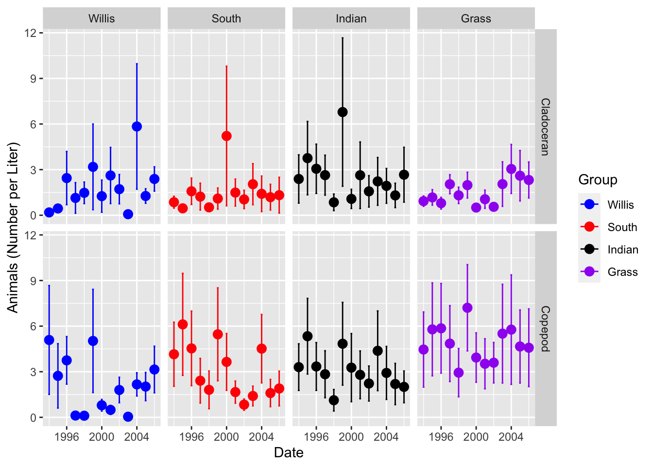
# So what if you wanted to see Cladoceran on the bottom?
lakes.df <- lakes.df %>%
  mutate(
    group = fct_relevel(group,
                            "Copepod", "Cladoceran"))
# here is an example of where you might want it...
# we can offset the points so they dont overlap
lakes.df %>% ggplot(aes(year, color = lake_name)) +
stat_summary(aes(y = org_l),
fun.y = mean, na.rm = TRUE,
geom = "point",
size = 3,
position = position_dodge(0.2)) +
stat_summary(aes(y = org_l),
fun.data = mean_se, na.rm = TRUE,
geom = "errorbar",
width = 0.2,
position = position_dodge(0.2)) +
labs(x = "Date", y = "Animals (Number per Liter)") +
scale_color_manual(name = "Group",
values = c("blue", "red", "black", "purple"),
labels = c("Willis", "South", "Indian", "Grass")) +
facet_grid(group ~ lake_name)## Warning: `fun.y` is deprecated. Use `fun` instead.