# Load Libraries ----
# this is done each time you run a script
library("readxl") # read in excel files
library("tidyverse") # dplyr and piping and ggplot etc
library("lubridate") # dates and times
library("scales") # scales on ggplot ases
library("skimr") # quick summary stats
library("janitor") # clean up excel imports
library("patchwork") # multipanel graphs
library("plotly")
##
## Attaching package: 'plotly'
## The following object is masked from 'package:ggplot2':
##
##     last_plot
## The following object is masked from 'package:stats':
##
##     filter
## The following object is masked from 'package:graphics':
##
##     layout
# read in file ----
lakes.df <- read_csv("data/Reduced_Lake_Long_Genus_Species.csv")
##
## ── Column specification ────────────────────────────────────────────────────────
## cols(
##   permanent_id = col_double(),
##   lake_name = col_character(),
##   date = col_date(format = ""),
##   group = col_character(),
##   genus_species = col_character(),
##   org_l = col_double(),
##   year = col_double()
## )
# Lets say we want to look at the data and figure out where outliers are

# I personally like to see what I am doing first
# lets look at only Cladocerans first
lakes.df %>%
  filter(group=='Cladoceran') %>%
  ggplot(aes(lake_name, org_l, color=group)) +
  geom_point(
  )
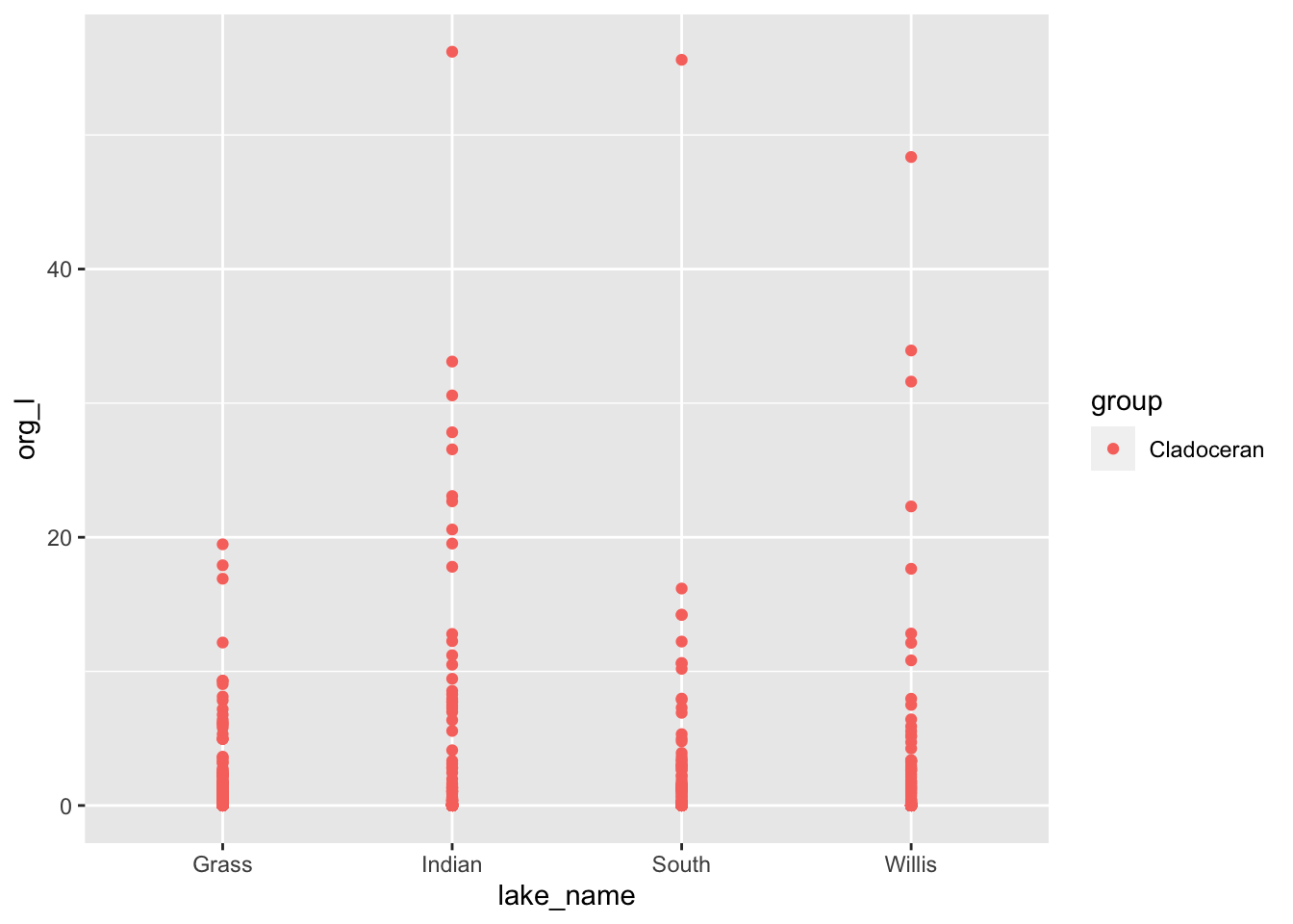
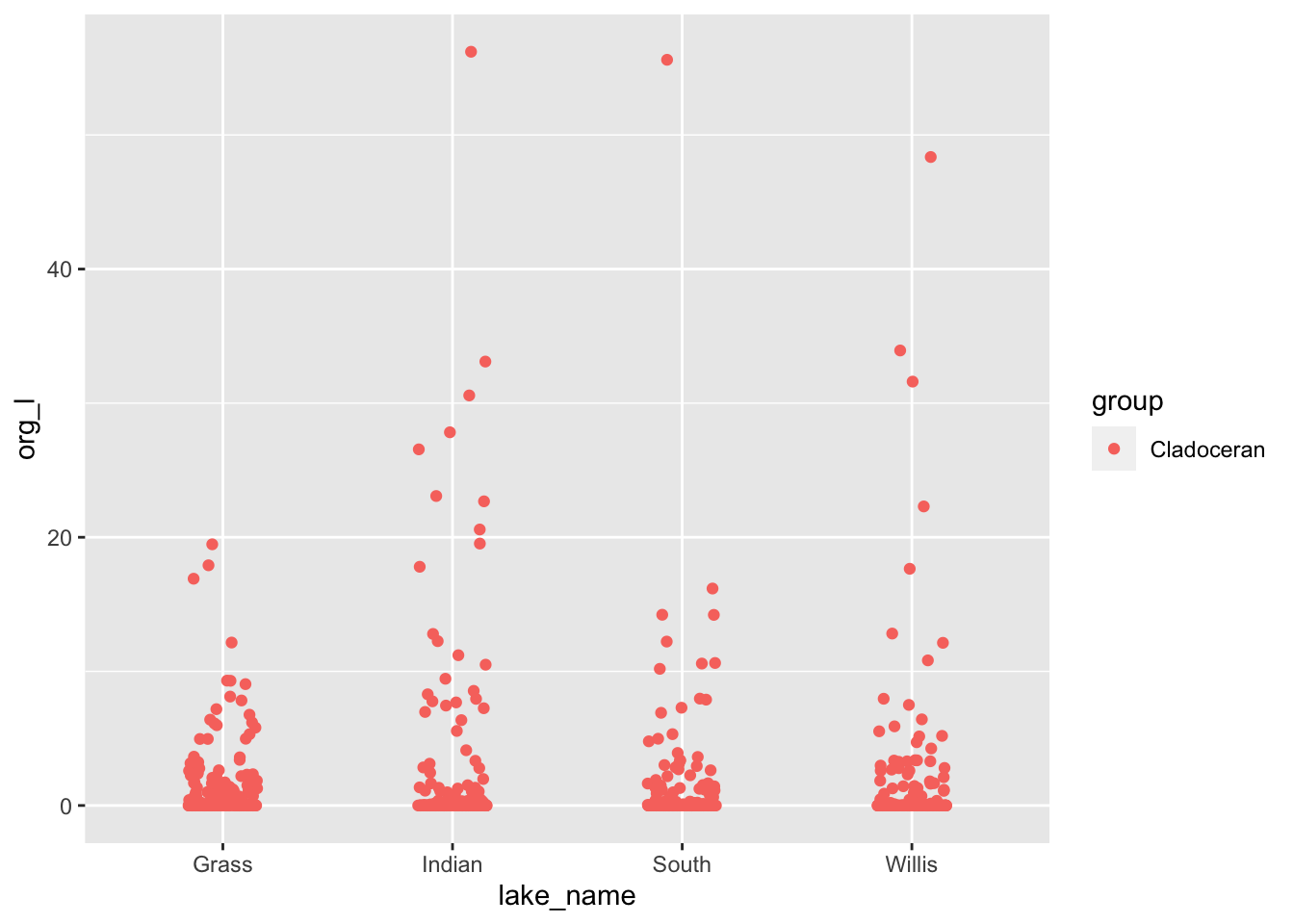
# Points overlap and you might want to spread them out a bit
lakes.df %>%
  filter(group=='Cladoceran') %>%
  ggplot(aes(lake_name, org_l, color=group)) +
  geom_point(
    position= position_jitterdodge(jitter.width = 0.3)
  )

# There are some high values - how can we figure out what they are...
# there are a few aproaches
clad.plot <- lakes.df %>%
  filter(group=='Cladoceran') %>%
  ggplot(aes(lake_name, org_l, color=group)) +
  geom_point(
    position= position_jitterdodge(jitter.width = 0.3)
  )
clad.plot
# I personally like the plotly package and GGPlotly
clad.plot <- lakes.df %>%
  filter(group=='Cladoceran') %>%
  ggplot(aes(lake_name, org_l, color=group, date=date, lake_name = lake_name, genus_species= genus_species)) +
  geom_point(
    position= position_jitterdodge(jitter.width = 0.1)
  )
clad.plot
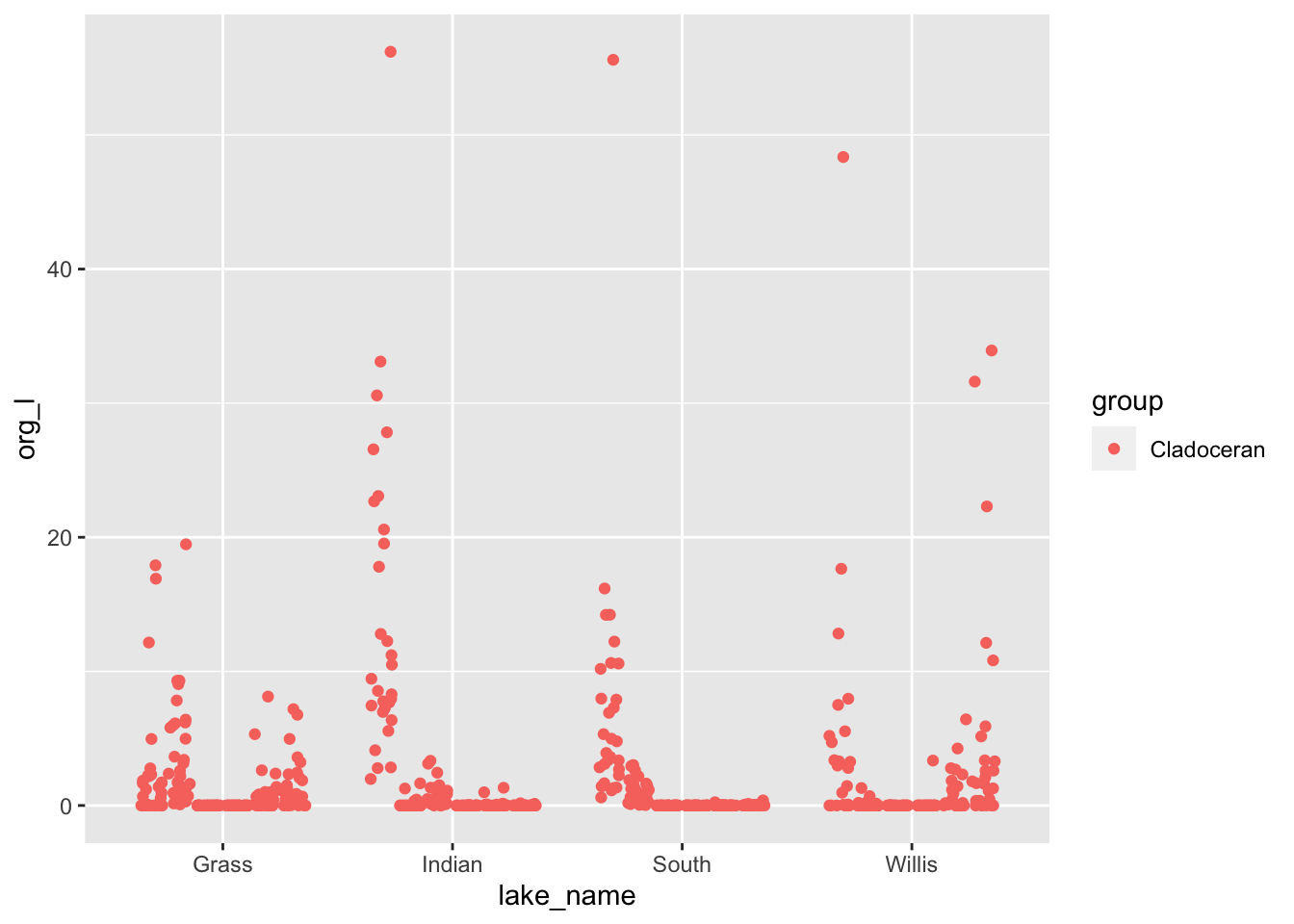
ggplotly(clad.plot, tooltip = c("date", "genus_species"))
# We could also do this by looking at the values that are above some threshold
# Display values greater than a value by group ------

lakes.df %>% group_by(lake_name) %>%
  filter(org_l > 40)
## # A tibble: 8 x 7
## # Groups:   lake_name [4]
##   permanent_id lake_name date       group      genus_species         org_l  year
##          <dbl> <chr>     <date>     <chr>      <chr>                 <dbl> <dbl>
## 1     47723283 Willis    1994-07-27 Copepod    Tropocyclops_extensus  57.3  1994
## 2     47723283 Willis    2004-07-06 Cladoceran Bosmina_longirostris   48.4  2004
## 3    131845587 Grass     1995-06-13 Copepod    Leptodiaptomus_minut…  46.1  1995
## 4    131845587 Grass     1996-06-18 Copepod    Leptodiaptomus_minut…  44.4  1996
## 5    131845587 Grass     2004-07-13 Copepod    Leptodiaptomus_minut…  41.2  2004
## 6    131845836 Indian    1999-06-29 Cladoceran Bosmina_longirostris   56.2  1999
## 7    131846593 South     2000-07-18 Cladoceran Bosmina_longirostris   55.6  2000
## 8    131846593 South     1995-09-13 Copepod    Leptodiaptomus_minut…  56.0  1995
# Using multiple conditions
lakes.df %>% group_by(lake_name) %>%
  filter(org_l > 40 & lake_name == "Willis")
## # A tibble: 2 x 7
## # Groups:   lake_name [1]
##   permanent_id lake_name date       group      genus_species         org_l  year
##          <dbl> <chr>     <date>     <chr>      <chr>                 <dbl> <dbl>
## 1     47723283 Willis    1994-07-27 Copepod    Tropocyclops_extensus  57.3  1994
## 2     47723283 Willis    2004-07-06 Cladoceran Bosmina_longirostris   48.4  2004
# or yes you can use or as |
lakes.df %>% group_by(lake_name) %>%
  filter(org_l > 40 & lake_name == "Willis" |
         org_l > 40 & lake_name == "South" )
## # A tibble: 4 x 7
## # Groups:   lake_name [2]
##   permanent_id lake_name date       group      genus_species         org_l  year
##          <dbl> <chr>     <date>     <chr>      <chr>                 <dbl> <dbl>
## 1     47723283 Willis    1994-07-27 Copepod    Tropocyclops_extensus  57.3  1994
## 2     47723283 Willis    2004-07-06 Cladoceran Bosmina_longirostris   48.4  2004
## 3    131846593 South     2000-07-18 Cladoceran Bosmina_longirostris   55.6  2000
## 4    131846593 South     1995-09-13 Copepod    Leptodiaptomus_minut…  56.0  1995
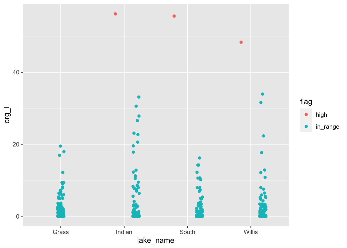
# Flagging data -----
# First the ifelse statement

lakes.df <- lakes.df %>%
  mutate(flag = ifelse(org_l >40, "high", "in_range"))
# Look at data...
lakes.df %>%
  filter(group=='Cladoceran') %>%
  ggplot(aes(lake_name, org_l, color=flag)) +
  geom_point(
    position= position_jitterdodge(jitter.width = 0.1)
  )
# Case_when ------
# you can nest if_else statements can be a mess
# this is where case_when comes into play
# this is the same but you can add more conditions easier
lakes.df <- lakes.df %>%
  mutate(flag = case_when(org_l > 40 ~ "high",
                          TRUE ~ "in_range"))
lakes.df <- lakes.df %>%
  mutate(flag = case_when(org_l > 40 ~ "high",
                          org_l < 40 & org_l >=30 ~ "medium",
                          org_l < 30 & org_l >=20 ~ "lower",
                          TRUE ~ "in_range"))