Ttests

T Tests

##Load libraries We will read in the main files and load the libraries as we have worked with so far.

# One new package for summary stats
#install.packages("broom")
# install.packages("GGally")
# install.packages("car")
# install.packages("gvlma")


# load the libraries each time you restart R
library(tidyverse)
library(lubridate)
library(scales)
library(skimr)
library(janitor)
library(patchwork)
# library(reshape2)
library(broom)
library(GGally)
library(corrplot)
library(car)

Read in file

# read in the file
iris.df <- read_csv("data/iris.csv") %>%
  clean_names() %>%
  remove_empty(c("rows", "cols")) 

## 
## ── Column specification ────────────────────────────────────────────────────────
## cols(
##   Sepal.Length = col_double(),
##   Sepal.Width = col_double(),
##   Petal.Length = col_double(),
##   Petal.Width = col_double(),
##   Species = col_character()
## )

glimpse(iris.df)

## Rows: 150
## Columns: 5
## $ sepal_length <dbl> 5.1, NA, 4.7, 4.6, 5.0, 5.4, 4.6, 5.0, 4.4, 4.9, 5.4, 4.8…
## $ sepal_width  <dbl> 3.5, 3.0, 3.2, 3.1, 3.6, 3.9, 3.4, 3.4, 2.9, 3.1, 3.7, 3.…
## $ petal_length <dbl> 1.4, 1.4, 1.3, 1.5, 1.4, 1.7, 1.4, 1.5, 1.4, 1.5, 1.5, 1.…
## $ petal_width  <dbl> 0.2, 0.2, 0.2, 0.2, 0.2, 0.4, 0.3, 0.2, 0.2, 0.1, 0.2, 0.…
## $ species      <chr> "setosa", "setosa", "setosa", "setosa", "setosa", "setosa…

###Summary Statistics for the better look ###So this is a lot different than thinking about data from excel
Lets try to do the summary stats on the data now and see how it differs

# the data you want to look at
skim(iris.df)

Data summary

Name	iris.df
Number of rows	150
Number of columns	5
_______________________
Column type frequency:
character	1
numeric	4
________________________
Group variables	None

Variable type: character

skim_variable	n_missing	complete_rate	min	max	empty	n_unique	whitespace
species	0	1	6	10	0	3	0

Variable type: numeric

skim_variable	n_missing	complete_rate	mean	sd	p0	p25	p50	p75	p100	hist
sepal_length	1	0.99	5.85	0.83	4.3	5.1	5.80	6.4	7.9	▆▇▇▅▂
sepal_width	0	1.00	3.06	0.44	2.0	2.8	3.00	3.3	4.4	▁▆▇▂▁
petal_length	0	1.00	3.76	1.77	1.0	1.6	4.35	5.1	6.9	▇▁▆▇▂
petal_width	0	1.00	1.20	0.76	0.1	0.3	1.30	1.8	2.5	▇▁▇▅▃

iris.df %>% group_by(species) %>% skim_to_wide()

## Warning: 'skim_to_wide' is deprecated.
## Use 'skim()' instead.
## See help("Deprecated")

Data summary

Name	.data
Number of rows	150
Number of columns	5
_______________________
Column type frequency:
numeric	4
________________________
Group variables	species

Variable type: numeric

skim_variable	species	n_missing	complete_rate	mean	sd	p0	p25	p50	p75	p100	hist
sepal_length	setosa	1	0.98	5.01	0.36	4.3	4.80	5.00	5.20	5.8	▃▃▇▅▁
sepal_length	versicolor	0	1.00	5.94	0.52	4.9	5.60	5.90	6.30	7.0	▂▇▆▃▃
sepal_length	virginica	0	1.00	6.59	0.64	4.9	6.23	6.50	6.90	7.9	▁▃▇▃▂
sepal_width	setosa	0	1.00	3.43	0.38	2.3	3.20	3.40	3.68	4.4	▁▃▇▅▂
sepal_width	versicolor	0	1.00	2.77	0.31	2.0	2.52	2.80	3.00	3.4	▁▅▆▇▂
sepal_width	virginica	0	1.00	2.97	0.32	2.2	2.80	3.00	3.18	3.8	▂▆▇▅▁
petal_length	setosa	0	1.00	1.46	0.17	1.0	1.40	1.50	1.58	1.9	▁▃▇▃▁
petal_length	versicolor	0	1.00	4.26	0.47	3.0	4.00	4.35	4.60	5.1	▂▂▇▇▆
petal_length	virginica	0	1.00	5.55	0.55	4.5	5.10	5.55	5.88	6.9	▃▇▇▃▂
petal_width	setosa	0	1.00	0.25	0.11	0.1	0.20	0.20	0.30	0.6	▇▂▂▁▁
petal_width	versicolor	0	1.00	1.33	0.20	1.0	1.20	1.30	1.50	1.8	▅▇▃▆▁
petal_width	virginica	0	1.00	2.03	0.27	1.4	1.80	2.00	2.30	2.5	▂▇▆▅▇

Wide to long format

# this will add an index to the dataframe so you know what individual is which
iris_long.df <- iris.df %>% 
  mutate(individual = row_number()) %>% 
  gather(trait, measure, -species, - individual)

head(iris_long.df)

## # A tibble: 6 x 4
##   species individual trait        measure
##   <chr>        <int> <chr>          <dbl>
## 1 setosa           1 sepal_length     5.1
## 2 setosa           2 sepal_length    NA  
## 3 setosa           3 sepal_length     4.7
## 4 setosa           4 sepal_length     4.6
## 5 setosa           5 sepal_length     5  
## 6 setosa           6 sepal_length     5.4

Outliers

# Box Plots of data
iris_long.df %>% group_by(species, trait) %>% 
  ggplot( aes(x = trait, y = measure, color = species, fill=species))+
  geom_boxplot(aes(alpha=0.3)) 

## Warning: Removed 1 rows containing non-finite values (stat_boxplot).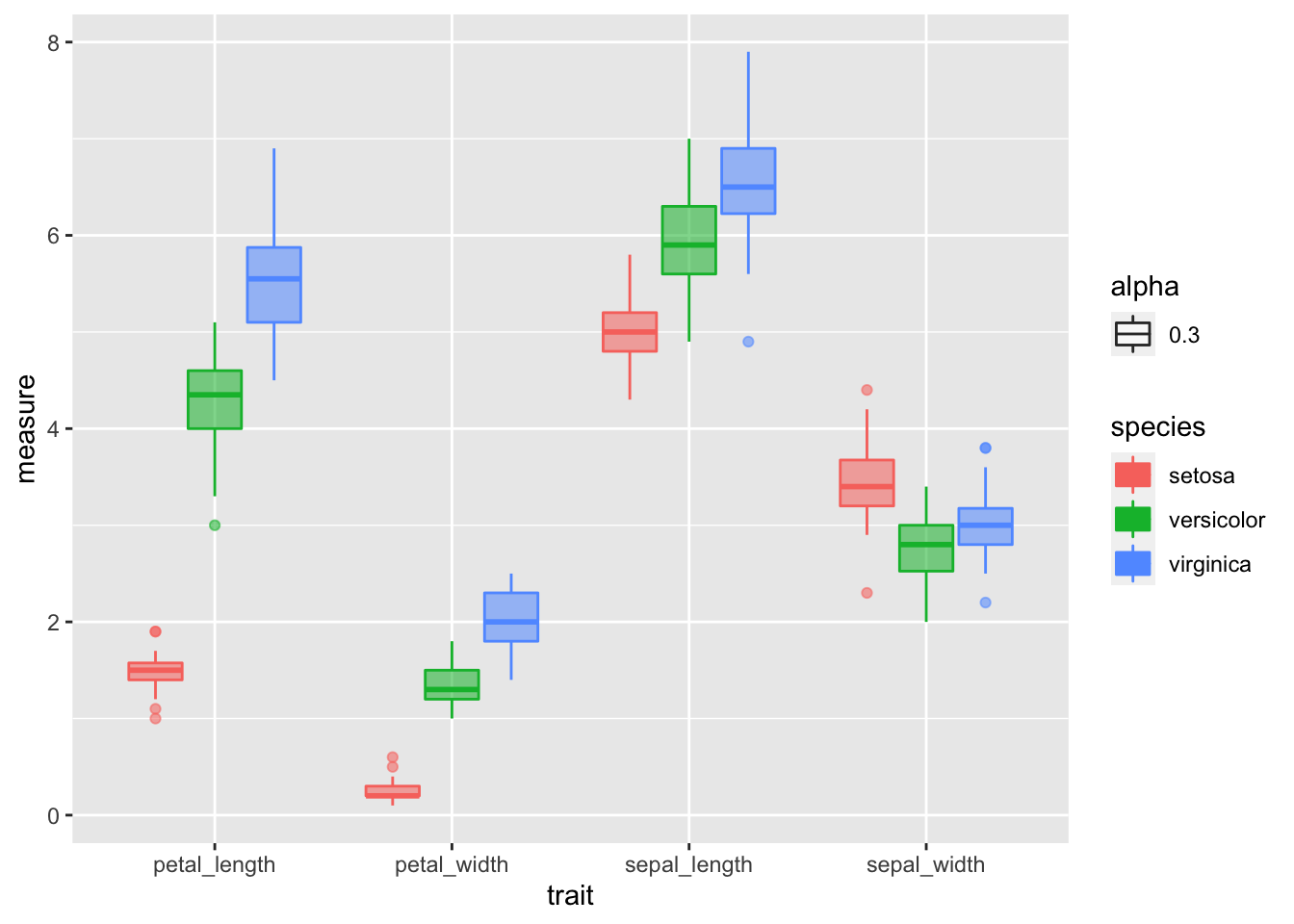

These look good for the most part with only one or two significant. Your choice to transform or not.

##Factors
Make sure the categorical variable is a factor
Rearrange the order of groups so that control group is first, followed by treatment groups.
you can do this by:

# Make Factors from the different levels long way
# iris_long.df$species <- as.factor(iris_long.df$species)  
# iris_long.df$trait <- as.factor(iris_long.df$trait) 

# Make Factors dplyr
iris_long.df <- iris_long.df %>%
  mutate(
    sex = factor(species, 
    labels = c("setosa", "versicolor", "virginica")),
    trait = factor(trait, 
    labels = c("sepal_length", "sepal_width", "petal_length", "petal_width"))
  )

Test for normality of data and using the broom package

So I think this is premature but some people like to test the normality of the data but really you should be assessing the normality of the residuals. But here it goes…

# turn off scientific notaton
options(scipen = 999)
# to turn back on 
#options(scipen = 0)

# Test for normality of each group and store in shapirowilktests
# This uses the broom package to get clean output of the test 
iris_long.df %>% group_by(species, trait) %>% do(tidy(shapiro.test(.$measure)))

## # A tibble: 12 x 5
## # Groups:   species, trait [12]
##    species    trait        statistic     p.value method                     
##    <chr>      <fct>            <dbl>       <dbl> <chr>                      
##  1 setosa     sepal_length     0.955 0.0548      Shapiro-Wilk normality test
##  2 setosa     sepal_width      0.800 0.000000866 Shapiro-Wilk normality test
##  3 setosa     petal_length     0.977 0.456       Shapiro-Wilk normality test
##  4 setosa     petal_width      0.972 0.272       Shapiro-Wilk normality test
##  5 versicolor sepal_length     0.966 0.158       Shapiro-Wilk normality test
##  6 versicolor sepal_width      0.948 0.0273      Shapiro-Wilk normality test
##  7 versicolor petal_length     0.978 0.465       Shapiro-Wilk normality test
##  8 versicolor petal_width      0.974 0.338       Shapiro-Wilk normality test
##  9 virginica  sepal_length     0.962 0.110       Shapiro-Wilk normality test
## 10 virginica  sepal_width      0.960 0.0870      Shapiro-Wilk normality test
## 11 virginica  petal_length     0.971 0.258       Shapiro-Wilk normality test
## 12 virginica  petal_width      0.967 0.181       Shapiro-Wilk normality test

#You can do this on all variables faster with if there was only one grouping
# tapply(iris_long.df$measure, iris_long.df$species, shapiro.test)

##Test for homogenetiy of variances

Best to use the Levenes test compared to the Bartlet test
uses the car package

http://www.cookbook-r.com/Statistical_analysis/Homogeneity_of_variance/

Note however that this is doing the homogeneity test on all traits and not each one which is what you really should do and is not often done. Need to check on this though.

#Test for homogeneity of variances by groups
leveneTest(sepal_length ~ species, data=iris.df)

## Warning in leveneTest.default(y = y, group = group, ...): group coerced to
## factor.

## Levene's Test for Homogeneity of Variance (center = median)
##        Df F value   Pr(>F)   
## group   2  6.0386 0.003022 **
##       146                    
## ---
## Signif. codes:  0 '***' 0.001 '**' 0.01 '*' 0.05 '.' 0.1 ' ' 1

#Compared to the Bartlet test
bartlett.test(sepal_length ~ species, data=iris.df)

## 
##  Bartlett test of homogeneity of variances
## 
## data:  sepal_length by species
## Bartlett's K-squared = 15.308, df = 2, p-value = 0.0004742

Create a subset dataframe

sepal_length.df <- iris_long.df %>%
  filter(trait =="sepal_length") %>%
  filter(species != "setosa")

If p-value >= 0.05, use var.equal=TRUE below

t.test(measure ~ species, data=sepal_length.df,
       var.equal=TRUE,
       conf.level=0.95)

## 
##  Two Sample t-test
## 
## data:  measure by species
## t = -12.604, df = 98, p-value < 0.00000000000000022
## alternative hypothesis: true difference in means between group versicolor and group virginica is not equal to 0
## 95 percent confidence interval:
##  -1.495426 -1.088574
## sample estimates:
## mean in group versicolor  mean in group virginica 
##                    4.260                    5.552

t.test(measure ~ species, data=sepal_length.df,
       var.equal=FALSE,
       conf.level=0.95)

## 
##  Welch Two Sample t-test
## 
## data:  measure by species
## t = -12.604, df = 95.57, p-value < 0.00000000000000022
## alternative hypothesis: true difference in means between group versicolor and group virginica is not equal to 0
## 95 percent confidence interval:
##  -1.49549 -1.08851
## sample estimates:
## mean in group versicolor  mean in group virginica 
##                    4.260                    5.552

Boxplot of data

sepal_length.df %>%
  ggplot(aes(species, measure, fill = species)) +
  geom_boxplot()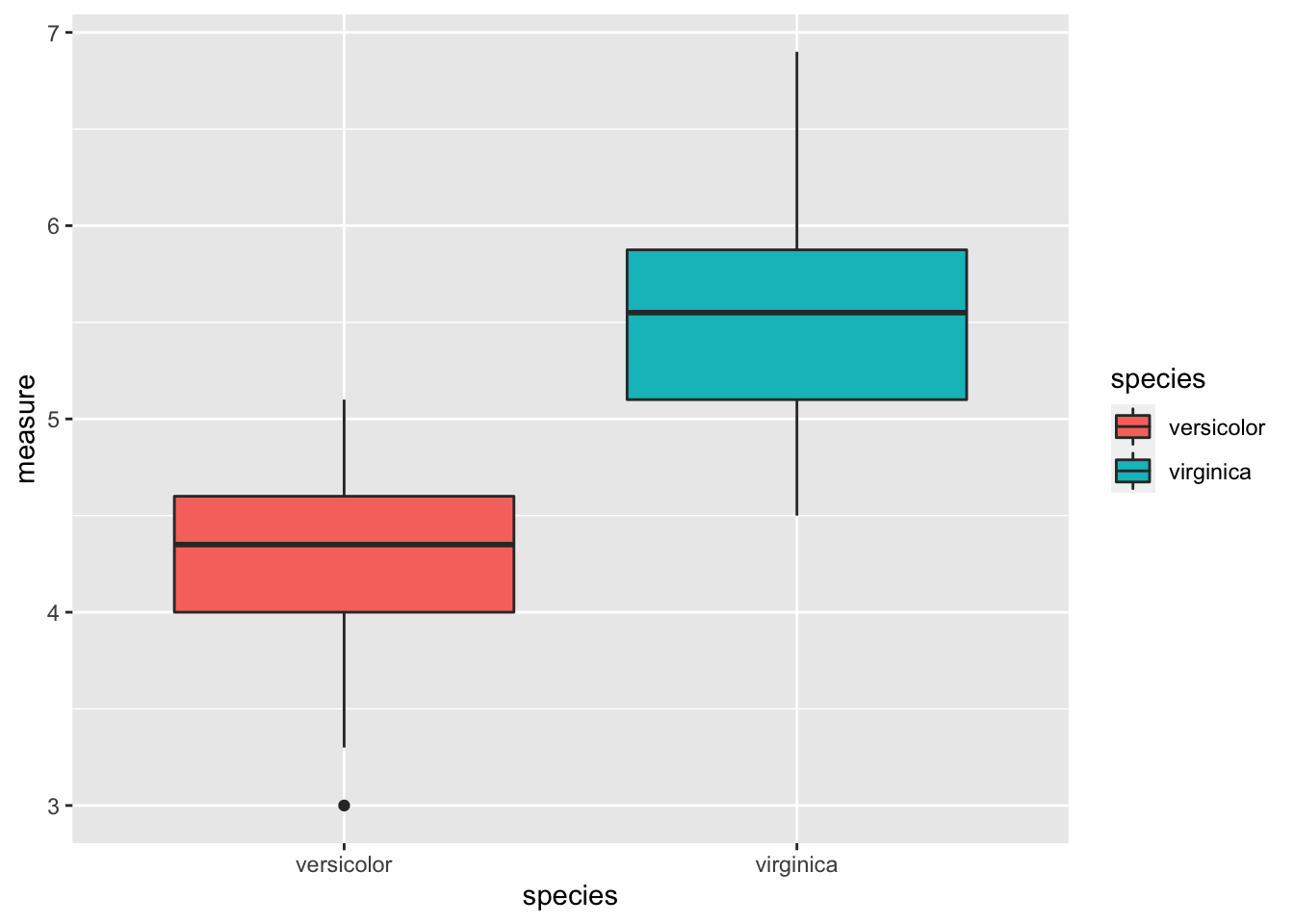

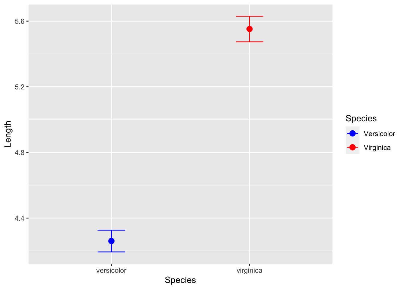
Mean and standard error plot

sepal_length.df %>% 
ggplot(aes(species, color=species)) + 
  stat_summary(aes(y = measure),
               fun.y = mean, na.rm = TRUE,
               geom = "point",
               size = 3) + 
  stat_summary(aes(y = measure),
               fun.data = mean_se, na.rm = TRUE,
               geom = "errorbar",
               width = 0.2) +
  labs(x = "Species", y = "Length") +
  scale_color_manual(name = "Species", 
                     values = c("blue", "red"),
                     labels = c("Versicolor", "Virginica"))

## Warning: `fun.y` is deprecated. Use `fun` instead.