Lecture: GLM & Logistic Regression

Generalized linear models

Generalized Linear Models (GLMs) for non-normal response data — Gaussian, Poisson, and negative binomial GLMs for count data, logistic regression for binary responses, odds ratios, model diagnostics, and the connection back to ANOVA.

Part 1 · Why the Linear Model Runs Out

Where We Left Off

Three weeks of linear models:

• One-way ANOVA
• Factorial ANOVA
• Nested ANOVA

Every one of them assumed:

• Normality of the residuals
• Homogeneity of variance — Levene’s or Bartlett’s
• Independence of observations

Important

Those assumptions are about the residuals, not the raw data — but when the response is a count or a yes/no, they fail in a way no transformation fully repairs.

Today: keep the linear part, change the distribution.

The Data: Galápagos Island Biogeography

The gala data — 29 Galápagos islands, MacArthur & Wilson’s island biogeography.

Column	What it is
spp	number of plant species — a count
endemics	number of endemic species — a count
area	island area, km²
elevation	maximum elevation, m

We bin area into size_cat so the predictor is categorical — the same shape of question as week 9.

Isabela is dropped: at ~4600 km² it is 20× anything else and flattens every plot.

count(g_df, size_cat)
##   size_cat  n
## 1    small 11
## 2   medium 12
## 3    large  6

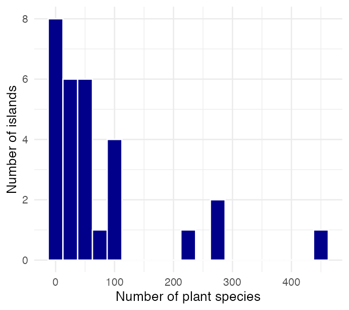
A Count Is Not a Normal Variable

A count has three properties a normal distribution does not:

1. It is a whole number
2. It cannot go below zero
3. Its variance grows with its mean

g_df %>%
  summarise(mean_spp = mean(spp),
            var_spp  = var(spp),
            ratio    = var_spp / mean_spp)
##   mean_spp  var_spp    ratio
## 1  76.2069 11078.46 145.3734

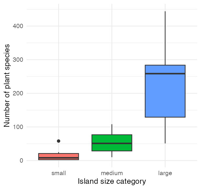
The variance is 145× the mean. A normal distribution is free to have any variance it likes, so that ratio is not itself a violation — but look at what it does to the groups.

Warning

The spread grows with the mean. That is the equal-variance assumption breaking, and it is the signature of count data.

Fit Last Week’s Model Anyway — and Watch It Fail

lm_model <- lm(spp ~ size_cat, data = g_df)

Anova(lm_model, type = 3)
## Anova Table (Type III tests)
## 
## Response: spp
##             Sum Sq Df F value     Pr(>F)    
## (Intercept)   2298  1  0.5069     0.4828    
## size_cat    192308  2 21.2064 0.00000345 ***
## Residuals   117889 26                       
## ---
## Signif. codes:  0 '***' 0.001 '**' 0.01 '*' 0.05 '.' 0.1 ' ' 1

shapiro.test(residuals(lm_model))$p.value
## [1] 0.000240339
leveneTest(spp ~ size_cat, data = g_df)$`Pr(>F)`[1]
## [1] 0.0005878942

Important

The p-value is 0.0000035. The model did not earn it.

• Normality of residuals: p < 0.001
• Equal variance: p < 0.001

Both assumptions fail, and they fail badly — not marginally.

The question is not wrong. Island size almost certainly does drive species richness. The model being used to answer it is making promises the data does not keep.

A normal 95% interval on the small islands predicts negative species counts.

What a GLM Changes

A generalized linear model keeps the linear part — \(\beta_0 + \beta_1 X_1 + \dots\) — and swaps out two things.

Component	What it is	Example
Random	the response’s distribution	Poisson for counts
Systematic	the predictors	size_cat, area
Link	connects the mean to the predictors	log for counts

\[g(\mu) = \beta_0 + \beta_1X_1 + \beta_2X_2 \dots\]

GLMs are fitted by maximum likelihood (ML), not ordinary least squares (OLS) — which is why their output talks about deviance rather than sums of squares.

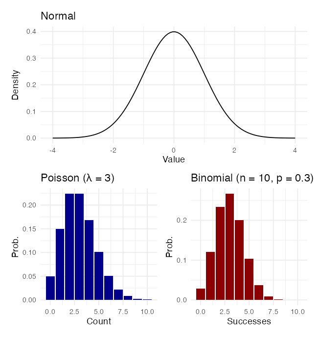
Choosing the Family and the Link

What the response looks like

Response	Family
continuous, symmetric	gaussian — this is lm()
counts	poisson
counts, variance > mean	negative binomial (glm.nb)
binary — present/absent	binomial(link = "logit")
positive, continuous, skewed	Gamma

The link function

Distribution	Link	Formula
Normal	Identity	\(g(\mu) = \mu\)
Poisson	Log	\(g(\mu) = \log(\mu)\)
Binomial	Logit	\(g(\mu) = \log[\mu/(1-\mu)]\)
Gamma	Log	\(g(\mu) = \log(\mu)\)

Tip

The link is what keeps predictions possible. A log link cannot predict a negative count. A logit link cannot predict a probability above 1.

Part 2 · Gaussian GLMs — the Sanity Check

Before Trusting glm(), Check It Against What You Know

Before handing glm() an unfamiliar distribution, confirm it reproduces the model you already trust.

A Gaussian family with an identity link is a linear model — same estimates, same standard errors, same p-values. If that does not come out identical, you have mis-specified something.

Note

You are not learning a new model. You are learning two arguments on the one you already have: family = and link =. Everything that follows today changes exactly those two.

Gaussian GLM — Same Model, Two Function Calls

gauss_model <- glm(spp ~ size_cat,
                   data = g_df,
                   family = gaussian(link = "identity"))

round(cbind(lm  = coef(lm_model),
            glm = coef(gauss_model)), 6)
##                       lm       glm
## (Intercept)     14.45454  14.45454
## size_catmedium  40.62879  40.62879
## size_catlarge  217.21212 217.21212

all.equal(coef(lm_model), coef(gauss_model))
## [1] TRUE

Anova(gauss_model, type = "III", test = "F")
## Analysis of Deviance Table (Type III tests)
## 
## Response: spp
## Error estimate based on Pearson residuals 
## 
##           Sum Sq Df F values     Pr(>F)    
## size_cat  192308  2   21.206 0.00000345 ***
## Residuals 117889 26                        
## ---
## Signif. codes:  0 '***' 0.001 '**' 0.01 '*' 0.05 '.' 0.1 ' ' 1

Identical to the Anova() on lm_model from Part 1 — F = 21.21, p = 0.0000035, and identical for the same reason: it is that model.

Gaussian GLM — Reading the New Vocabulary

##       GLM summary says    value       ANOVA calls it
## 1 Dispersion parameter   4534.2 Residual mean square
## 2        Null deviance 310196.8             SS total
## 3    Residual deviance 117889.0          SS residual
## 4      null - residual 192307.8          SS size_cat

A GLM summary renames three things you already know:

• Dispersion parameter — for a Gaussian GLM this is the residual variance, \(\sigma^2\). It is the ANOVA table’s residual mean square.

• Null deviance — the error left when you predict every island with the grand mean alone. For a Gaussian GLM this is SS_total.

• Residual deviance — the error left after fitting size_cat. For a Gaussian GLM this is SS_residual.

Important

Null deviance − residual deviance = the model sum of squares. The residual deviance is the part your predictor did not explain.

Part 3 · Poisson GLMs for Count Data

The Poisson Distribution and Its One Strong Claim

Poisson is the distribution for counts:

• Number of species on an island
• Number of parasites in a host
• Number of nests in a plot

It assumes:

• Counts are non-negative integers
• Events occur independently
• The mean equals the variance

That third one is not a convenience. Poisson has only one parameter, λ, which is simultaneously its mean and its variance. You do not get to set them separately.

Warning

Remember the ratio. The variance of spp is 145× its mean.

Poisson insists that ratio is 1.

Fit it anyway — the failure is the content.

Tip

Why log is the link. \(\log(\mu)\) runs from −∞ to +∞, so the linear predictor can be any number at all and \(\mu = e^{\eta}\) is still positive. Counts can never come out negative.

Fitting the Poisson GLM

poiss_model <- glm(spp ~ size_cat,
                   data = g_df,
                   family = poisson(link = "log"))

round(summary(poiss_model)$coefficients, 4)
##                Estimate Std. Error z value Pr(>|z|)
## (Intercept)      2.6710     0.0793 33.6804        0
## size_catmedium   1.3378     0.0883 15.1460        0
## size_catlarge    2.7743     0.0837 33.1387        0

The model predicts the natural log of the expected count, so exponentiate to read it:

• \(e^{2.671} = 14.5\) species on a small island
• \(e^{1.338} = 3.81\) — a medium island has 3.8× the species of a small one
• \(e^{2.774} = 16.0\) — a large island has 16× the species of a small one

Important

With a log link, coefficients are multiplicative, not additive. A coefficient of β multiplies the mean by \(e^{\beta}\).

Testing the Effect — Why LR and Not F

Anova(poiss_model, type = "III", test = "LR")
## Analysis of Deviance Table (Type III tests)
## 
## Response: spp
##          LR Chisq Df            Pr(>Chisq)    
## size_cat   2133.2  2 < 0.00000000000000022 ***
## ---
## Signif. codes:  0 '***' 0.001 '**' 0.01 '*' 0.05 '.' 0.1 ' ' 1

• An ANOVA F-test is a ratio of variances, and its denominator is the residual mean square — an estimate of \(\sigma^2\).

• A Poisson GLM never estimates a \(\sigma^2\). The variance is not a free parameter; it is pinned to the mean. There is nothing to put in the denominator.

• So we use a likelihood ratio (LR) test instead: fit the model with size_cat and the model without it, and compare how much better the full model explains the data.

\[\text{LR } \chi^2 = 2(\log L_{full} - \log L_{reduced})\]

Hold on to that 2133.2. It is about to shrink by a factor of 43.

Three Ways to Say “Log” — and Why They Differ

Model	R code	Interpretation of β₁
GLM, log link	glm(Y ~ X, family = poisson)	A 1-unit change in X multiplies the mean of Y by \(e^{\beta_1}\)
lm on logged Y	lm(log(Y) ~ X)	A 1-unit change in X multiplies the median of Y by \(e^{\beta_1}\)
log-log	lm(log(Y) ~ log(X))	A 1% change in X gives a β₁% change in Y

Important

These are not the same model. A GLM with a log link models the log of the mean, \(\log(E[Y])\). Logging the response models the mean of the log, \(E[\log(Y)]\) — which back-transforms to a geometric mean, not an arithmetic one. The GLM also never has to decide what to do with a zero count.

Part 4 · Overdispersion and the Negative Binomial

Checking Dispersion — the Test That Matters

The dispersion parameter is observed variance over expected variance:

\[\hat\phi = \frac{\sum \text{(Pearson residual)}^2}{\text{residual df}}\]

• ≈ 1 — good fit, variance = mean
• > 1 — overdispersion, variance > mean
• < 1 — underdispersion

check_overdispersion(poiss_model)
## # Overdispersion test
## 
##        dispersion ratio =  33.525
##   Pearson's Chi-Squared = 871.642
##                 p-value = < 0.001

Warning

Dispersion ratio 33.5, not 1.

The model is claiming the variance of a large island’s species count is about 232 — because Poisson forces variance = mean. The data say it is 20,400.

⚠️ shapiro.test(residuals(poiss_model)) will run, and give you a number. The number is meaningless — normality of raw residuals is not a Poisson assumption.

R will not stop you running a test that does not apply. Check the diagnostic that matches the model, not the one you remember.

The DHARMa Residual Check

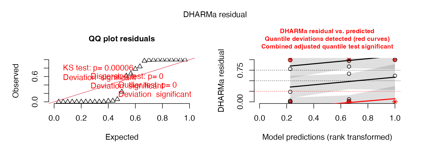
Ordinary GLM residuals are hard to read. DHARMa simulates from the fitted model and asks where each observation falls in its own predicted distribution — if the model is right, those are uniform. Here they are not, and the problem is not subtle.

The Negative Binomial — a Second Parameter

The negative binomial adds theta (θ), which lets the variance exceed the mean by as much as it needs to:

\[\operatorname{Var}(Y) = \mu + \frac{\mu^2}{\theta}\]

As θ → ∞ this collapses back to the Poisson. A small θ means a lot of extra spread.

nb_model <- glm.nb(spp ~ size_cat, data = g_df)

c(theta = nb_model$theta)
##    theta 
## 1.660219

check_overdispersion(nb_model)
## # Overdispersion test (using simulated residuals)
## 
##  dispersion ratio = 0.586
##           p-value = 0.632

Anova(nb_model, type = "III", test = "LR")
## Analysis of Deviance Table (Type III tests)
## 
## Response: spp
##          LR Chisq Df       Pr(>Chisq)    
## size_cat   49.858  2 0.00000000001491 ***
## ---
## Signif. codes:  0 '***' 0.001 '**' 0.01 '*' 0.05 '.' 0.1 ' ' 1

AIC(poiss_model, nb_model)
##             df       AIC
## poiss_model  3 1057.1686
## nb_model     4  283.9725

Note

The dispersion is gone, and the AIC drops by 773. Same data, same predictor, same link — the only thing added was permission for the variance to be larger than the mean.

What Overdispersion Did to Your p-Value

##                estimate SE_poisson SE_negbin
## (Intercept)      2.6710      0.079     0.247
## size_catmedium   1.3378      0.088     0.336
## size_catlarge    2.7743      0.084     0.403

	Poisson	Negative binomial
size_cat LR χ²	2133.2	49.9
dispersion ratio	33.5	0.59
AIC	1057.2	284.0

Important

Every coefficient is identical to four decimal places.

The two models put the means in exactly the same place. What changed is the standard errors — the Poisson’s are 3× to 5× too small, and the LR χ² is inflated 43-fold.

Overdispersion does not move your estimate. It makes you far more confident in it than you are entitled to be — smaller SEs, bigger test statistics, narrower intervals, smaller p-values.

Both models here say p < 0.001. The conclusion did not change. Only the honesty of it did — and that is still worth getting right, because the next dataset will be the one where it flips.

Estimated Marginal Means on the Count Scale

nb_emm <- emmeans(nb_model, ~ size_cat,
                  type = "response")
nb_emm
##  size_cat response    SE  df asymp.LCL asymp.UCL
##  small        14.5  3.57 Inf      8.91      23.5
##  medium       55.1 12.50 Inf     35.27      86.0
##  large       231.7 73.70 Inf    124.22     432.0
## 
## Confidence level used: 0.95 
## Intervals are back-transformed from the log scale

type = "response" back-transforms from the log scale, which is why the confidence limits are not symmetric around each mean — the interval was symmetric on the log scale, and exponentiating stretches the upper half.

##  size_cat response    SE  df asymp.LCL asymp.UCL .group
##  small        14.5  3.57 Inf      8.91      23.5  a    
##  medium       55.1 12.50 Inf     35.27      86.0   b   
##  large       231.7 73.70 Inf    124.22     432.0    c  
## 
## Confidence level used: 0.95 
## Intervals are back-transformed from the log scale 
## P value adjustment: tukey method for comparing a family of 3 estimates 
## Tests are performed on the log scale 
## significance level used: alpha = 0.05 
## NOTE: If two or more means share the same grouping symbol,
##       then we cannot show them to be different.
##       But we also did not show them to be the same.

Poisson vs. Negative Binomial, Drawn

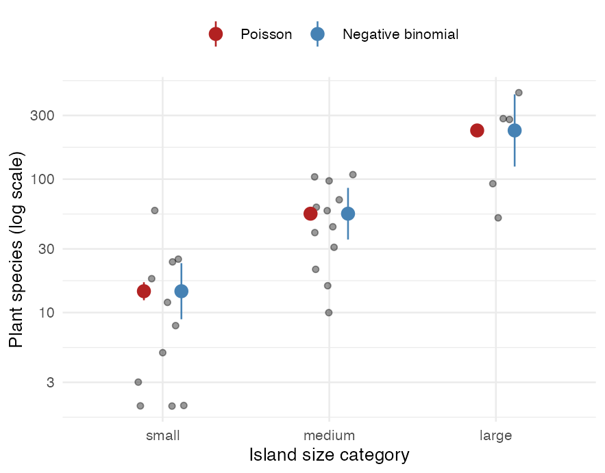
The means land on top of each other. Only the intervals differ.

For the large islands:

• Poisson: 232 (220 – 244)
• Negative binomial: 232 (124 – 432)

The Poisson interval is 24 species wide and excludes most of the observed data. The negative binomial interval is 308 species wide and actually contains it.

Tip

Report the one whose diagnostics pass, not the one with the smaller p-value.

Part 5 · Logistic Regression

A Binary Response Is the Other Kind of Non-Normal

A count was one kind of non-normal response. A yes/no is another — dead/alive, present/absent, infected/healthy.

Logistic regression models the probability that Y = 1:

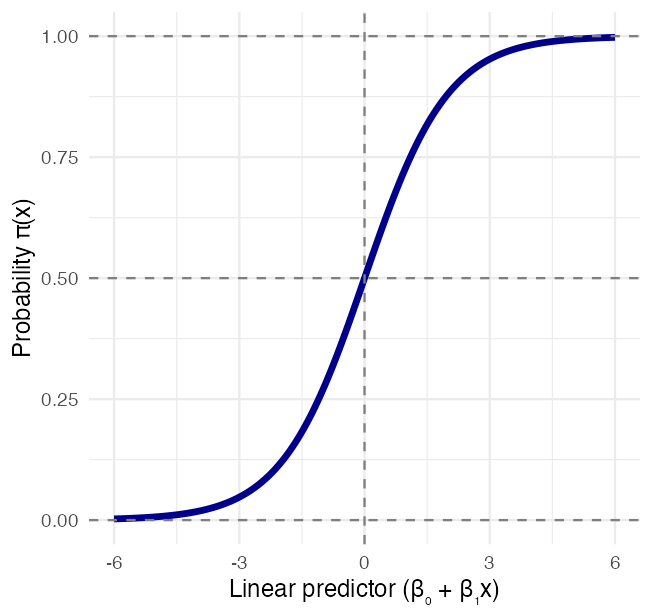
\[\pi(x) = \frac{e^{\beta_0 + \beta_1 x}}{1 + e^{\beta_0 + \beta_1 x}}\]

The logit link stretches probability — stuck between 0 and 1 — onto a scale that runs from −∞ to +∞:

\[g(x) = \log\left(\frac{\pi(x)}{1-\pi(x)}\right) = \beta_0 + \beta_1 x\]

The thing inside the log, \(\pi/(1-\pi)\), is the odds. So the linear model is a model of log-odds.

Note

Gotelli & Ellison, A Primer of Ecological Statistics, Ch. 11 — The Analysis of Categorical Data, for logistic regression and binomial GLMs.

The Polis Lizard Data

Polis et al. (1998) recorded whether the lizard Uta was present on 19 islands in the Gulf of California, against each island’s perimeter-to-area ratio — a measure of how exposed its shoreline is.

polis_df %>%
  dplyr::select(island, paratio, uta, pa) %>%
  head(5)
## # A tibble: 5 × 4
##   island     paratio uta      pa
##   <chr>        <dbl> <chr> <dbl>
## 1 Bota         15.4  P         1
## 2 Cabeza        5.63 P         1
## 3 Cerraja      25.9  P         1
## 4 Coronadito   15.2  A         0
## 5 Flecha       13.0  P         1

count(polis_df, uta)
## # A tibble: 2 × 2
##   uta       n
##   <chr> <int>
## 1 A         9
## 2 P        10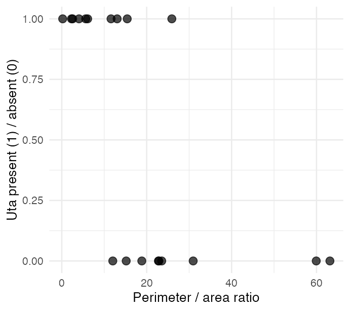

Note

These are the data from the paper, as reproduced in Quinn & Keough Box 13-1 — the same file the activity uses.

Fitting the Logistic Model

lizard_model <- glm(pa ~ paratio,
                    data = polis_df,
                    family = binomial(link = "logit"))

round(summary(lizard_model)$coefficients, 4)
##             Estimate Std. Error z value Pr(>|z|)
## (Intercept)   3.6061     1.6953  2.1272   0.0334
## paratio      -0.2196     0.1005 -2.1842   0.0289

Two ways to test \(H_0: \beta_1 = 0\):

1. Wald test — estimate / SE, the z column above
2. Likelihood ratio test — compare the full model to one with no predictor

null_model <- glm(pa ~ 1, data = polis_df,
                  family = binomial(link = "logit"))

anova(null_model, lizard_model, test = "Chisq")
## Analysis of Deviance Table
## 
## Model 1: pa ~ 1
## Model 2: pa ~ paratio
##   Resid. Df Resid. Dev Df Deviance  Pr(>Chi)    
## 1        18     26.287                          
## 2        17     14.221  1   12.066 0.0005134 ***
## ---
## Signif. codes:  0 '***' 0.001 '**' 0.01 '*' 0.05 '.' 0.1 ' ' 1

The LR test is the one to report — it is better behaved at small n, and 19 islands is small.

The Fitted Probability Curve

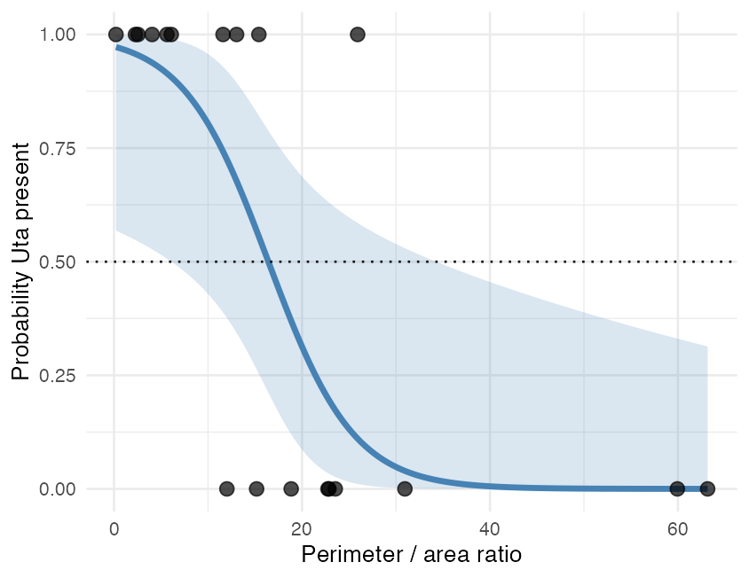
The curve crosses p = 0.5 at a perimeter-to-area ratio of

\[-\frac{\beta_0}{\beta_1} = -\frac{3.606}{-0.2196} = 16.4\]

Below that, Uta is more likely present than absent; above it, more likely absent.

Tip

The curve is the link doing its job. A straight line would have crossed below zero on the right of this plot and predicted a negative probability.

Interpreting the Odds Ratio

exp(coef(lizard_model))
## (Intercept)     paratio 
##  36.8210344   0.8028734

exp(confint(lizard_model, "paratio"))
##     2.5 %    97.5 % 
## 0.6157322 0.9356727

Odds ratio = \(e^{\beta_1}\)

• > 1 — raising the predictor raises the odds
• < 1 — raising the predictor lowers the odds
• = 1 — no effect

Here the odds ratio is 0.803:

• One extra unit of perimeter-to-area ratio multiplies the odds of finding Uta by 0.80
• That is a 19.7% drop in the odds per unit (1 − 0.803)
• The CI is 0.616 to 0.936 — entirely below 1, so the relationship is negative

Important

For an odds ratio the null value is 1, not 0 — it lives on a multiplicative scale. A CI that excludes 1 is the significant one.

Assessing Model Fit

# McFadden's, by hand
1 - lizard_model$deviance /
      lizard_model$null.deviance
## [1] 0.4590197

r2(lizard_model)   # performance's default
## # R2 for Logistic Regression
##   Tjur's R2: 0.521

hoslem.test(lizard_model$y,
            fitted(lizard_model), g = 10)
## 
##  Hosmer and Lemeshow goodness of fit (GOF) test
## 
## data:  lizard_model$y, fitted(lizard_model)
## X-squared = 7.898, df = 8, p-value = 0.4435

McFadden’s pseudo-R² = \(1 - \dfrac{D_{resid}}{D_{null}}\) = 0.459. performance::r2() instead reports Tjur’s R² = 0.521.

Both are “pseudo” because there is no residual variance to partition — the response is 0 or 1, so “proportion of variance explained” has nothing to be a proportion of. They are different quantities, so say which one you report. For McFadden’s, treat 0.2–0.4 as a strong model, not the 0.7 you would want from a regression.

Warning

Hosmer–Lemeshow runs backwards. Its null hypothesis is that the model fits. You want p large. Here p = 0.44, so there is no evidence of poor fit.

That is the opposite of every test you have run this semester — and it is why a “non-significant” result is not always bad news.

Part 6 · Multiple Logistic Regression

The Bolger Canyon Fragment Data

Logistic regression extends to several predictors exactly as regression does:

\[g(x) = \beta_0 + \beta_1 x_1 + \beta_2 x_2 + \ldots + \beta_p x_p\]

Bolger et al. (1997) recorded whether native rodents were present in 25 canyon fragments in coastal southern California, against three predictors.

Column	What it is
rodentsp	1 = rodents present, 0 = absent
pershrub	% shrub cover
distx	distance to source canyon, m
age	years since isolation

rodent_model <- glm(
  rodentsp ~ distx + age + pershrub,
  data = bolger_df,
  family = binomial(link = "logit"))

round(summary(rodent_model)$coefficients, 4)
##             Estimate Std. Error z value Pr(>|z|)
## (Intercept)  -5.9099     3.1125 -1.8987   0.0576
## distx         0.0003     0.0008  0.3988   0.6900
## age           0.0250     0.0377  0.6640   0.5067
## pershrub      0.0959     0.0406  2.3606   0.0182

Note

Quinn & Keough Box 13-2. Two predictors measure isolation (distx, age); one measures habitat quality (pershrub).

Testing Each Predictor

Anova(rodent_model, type = "II", test = "LR")
## Analysis of Deviance Table (Type II tests)
## 
## Response: rodentsp
##          LR Chisq Df Pr(>Chisq)   
## distx      0.1559  1   0.692943   
## age        0.4446  1   0.504906   
## pershrub   9.5577  1   0.001991 **
## ---
## Signif. codes:  0 '***' 0.001 '**' 0.01 '*' 0.05 '.' 0.1 ' ' 1

Each row drops one predictor and compares the two models by likelihood ratio — the multi-predictor version of what we did to the lizard model.

##              OR  2.5 % 97.5 %
## distx    1.0003 0.9986 1.0019
## age      1.0253 0.9495 1.1123
## pershrub 1.1006 1.0311 1.2249

Important

Shrub cover is the only one that matters. Each extra percentage point of shrub cover multiplies the odds of rodent presence by 1.10 (CI 1.03–1.22).

Neither isolation measure comes close — and both of their CIs bracket 1.

Visualizing Each Effect

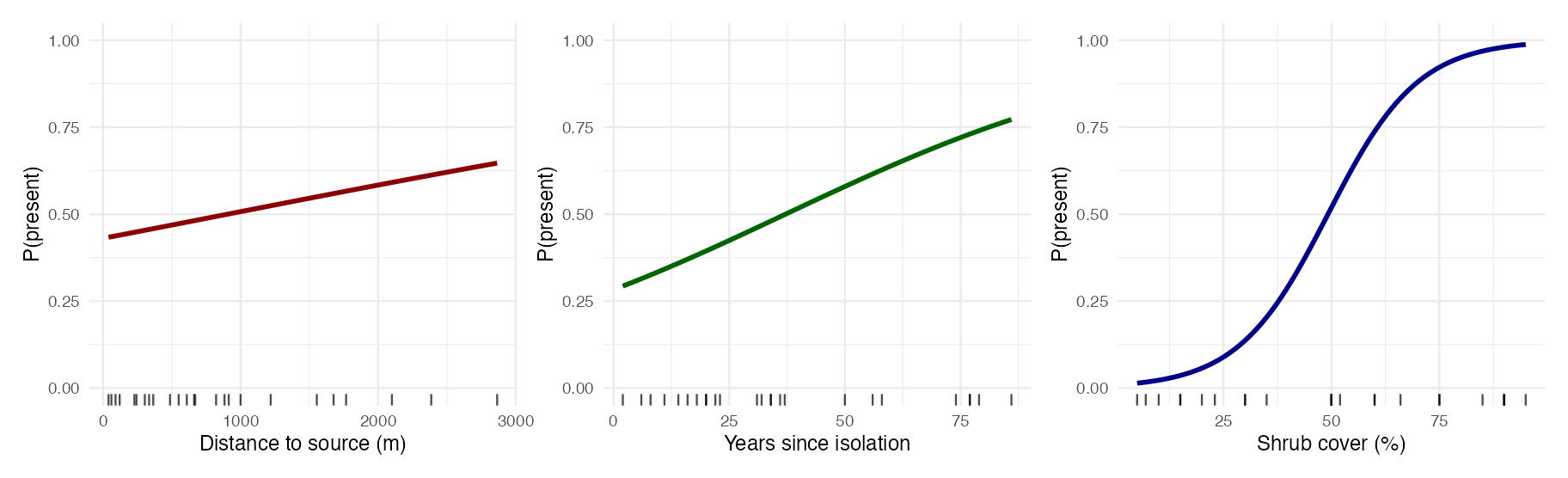
Each panel moves one predictor across its observed range and holds the other two at their means. Only shrub cover takes the probability from near 0 to near 1.

Model Comparison and Selection

##            Model k   AIC Deviance
## 1     Shrub only 2 24.05    20.05
## 2    No distance 3 25.51    19.51
## 3         No age 3 25.80    19.80
## 4           Full 4 27.36    19.36
## 5       No shrub 3 34.92    28.92
## 6 Intercept only 1 36.62    34.62

• Likelihood ratio tests compare nested models — one must be a special case of the other
• AIC / BIC compare any models fitted to the same data, nested or not
• AIC rewards fit and penalises parameters: \(AIC = -2\log L + 2k\)

Note

Dropping distx or age improves the AIC — they were costing a parameter each and buying almost nothing. Dropping pershrub makes it far worse.

How Well Does It Classify?

pred_prob  <- predict(rodent_model, type = "response")
pred_class <- ifelse(pred_prob > 0.5, 1, 0)

cm <- table(Predicted = pred_class,
            Actual = bolger_df$rodentsp)
cm
##          Actual
## Predicted  0  1
##         0 11  3
##         1  2  9

round(c(accuracy    = sum(diag(cm)) / sum(cm),
        sensitivity = cm["1","1"] / sum(cm[, "1"]),
        specificity = cm["0","0"] / sum(cm[, "0"])), 3)
##    accuracy sensitivity specificity 
##       0.800       0.750       0.846

• Accuracy — fraction of fragments called correctly
• Sensitivity — of the fragments that had rodents, how many did we catch?
• Specificity — of the fragments that did not, how many did we correctly rule out?

Warning

The 0.5 cut-off is a choice, not a result. Move it and sensitivity and specificity trade against each other. Classification accuracy is also optimistic here — we are scoring the model on the same 25 fragments we fitted it to.

Publication-Quality Figure

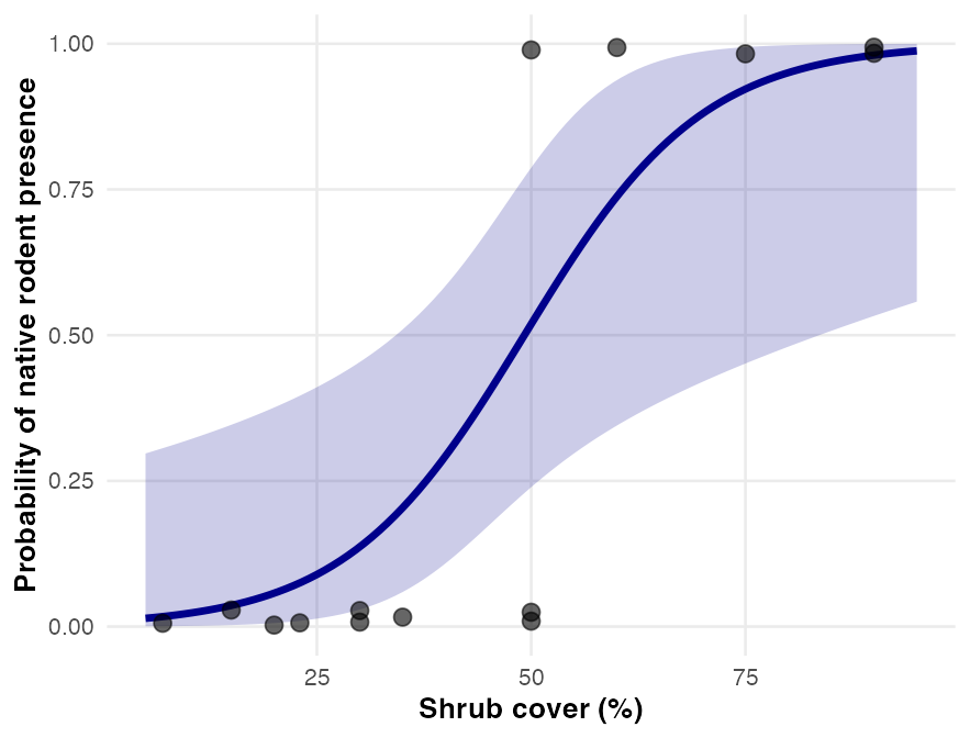
What makes this publishable rather than exploratory:

• The raw data are visible under the fit, jittered just enough to separate ties
• The confidence band is on the probability scale, computed on the link scale and back-transformed — so it can never leave [0, 1]
• Axis labels name the units, not the column names
• The other two predictors are held at their means, and the caption must say so

This is the shape of the graded figure in section 10 of the activity.

Scientific Write-Up — Results

ImportantResults

The presence of native rodents in 25 canyon fragments was modelled by multiple logistic regression with three predictors: distance to the nearest source canyon, years since isolation, and percentage shrub cover. The three predictors together improved substantially on the null model (likelihood-ratio χ² = 15.26, df = 3, p = 0.002; McFadden’s R² = 0.44).

Shrub cover was the only predictor with a detectable effect (β = 0.096, SE = 0.041, LR χ² = 9.56, df = 1, p = 0.002). Each additional percentage point of shrub cover multiplied the odds of rodent presence by 1.10 (95% CI 1.03–1.22). Neither distance to the source canyon (LR χ² = 0.16, p = 0.69) nor years since isolation (LR χ² = 0.44, p = 0.50) was distinguishable from zero.

The model classified 80% of fragments correctly (sensitivity 0.75, specificity 0.85) and showed no evidence of lack of fit (Hosmer–Lemeshow χ² = 6.04, df = 8, p = 0.64).

Scientific Write-Up — Discussion

ImportantDiscussion

Vegetation structure, not isolation, predicted whether native rodents persisted in these canyon fragments. Shrub cover is plausibly acting as both food and cover from predators, and the effect is large enough to matter on the ground: holding distance and age at their means, a fragment at 70% shrub cover has an 88% chance of retaining its rodents, against 6% for one at 20%.

The two isolation measures showed no detectable relationship. With 25 fragments, failing to detect an effect is not the same as showing there is none — but the AIC comparison points the same way, since dropping either one improved the model. The practical reading is that within this range of fragment ages and distances, habitat quality dominates.

Part 7 · Diagnostics and Assumptions

Assumptions of Logistic Regression

1. Independence of observations
2. Linearity between each predictor and the log odds — not the probability
3. No extreme outliers or high-leverage points
4. No multicollinearity among predictors
5. Enough data per parameter — a rough rule is 10 events per predictor

Warning

Assumption 2 is the one people forget. Logistic regression does not assume a linear relationship with the probability — the curve is S-shaped by construction. It assumes linearity on the logit scale.

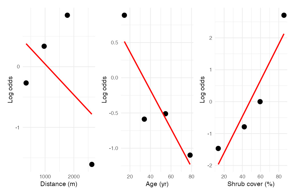
Bin each predictor, compute the empirical log-odds in each bin, and look for a straight line. Shrub cover is close to one; with 25 fragments these are rough.

Which Diagnostic for Which Family

Family	What it assumes	What to check
All GLMs	Independence; correct link; no extreme leverage	DHARMa residuals, Cook’s distance, VIF
Gaussian	Normal residuals, equal variance	shapiro.test(), Levene’s, residual plots
Poisson	Counts; variance = mean	check_overdispersion(), testDispersion()
Negative binomial	Counts; variance = \(\mu + \mu^2/\theta\)	check_overdispersion(), DHARMa
Binomial / logistic	Binary response; linear on the logit scale; enough events	Binned log-odds plot, Hosmer–Lemeshow, separation warnings

Important

Check the diagnostic that matches the model you fitted, not the one you learned first. shapiro.test() on Poisson residuals will give you a number, and the number will mean nothing.

Part 8 · GLMs, ANOVA, and Wrap-Up

One-Way ANOVA Is a Gaussian GLM

Every linear model you have fitted this semester is the special case of a GLM where:

1. The response is normal
2. The link is the identity

So a one-way ANOVA, a linear regression on a categorical predictor, and a Gaussian GLM are three names for one fit.

aov_fit  <- aov(spp ~ size_cat, data = g_df)
lm_fit   <- lm(spp ~ size_cat, data = g_df)
glm_fit  <- glm(spp ~ size_cat, data = g_df,
                family = gaussian(link = "identity"))

round(cbind(aov = coef(aov_fit),
            lm  = coef(lm_fit),
            glm = coef(glm_fit)), 4)
##                     aov       lm      glm
## (Intercept)     14.4545  14.4545  14.4545
## size_catmedium  40.6288  40.6288  40.6288
## size_catlarge  217.2121 217.2121 217.2121

c(aov = summary(aov_fit)[[1]][1, "F value"],
  lm  = anova(lm_fit)[1, "F value"])
##     aov      lm 
## 21.2064 21.2064

Note

Identical coefficients, identical F. GLMs did not replace the ANOVA — they contain it.

Summary — What a GLM Gives You

1. Gaussian + identity link = the linear model and ANOVA you already know
2. Poisson + log link = counts — and always check the dispersion
3. Negative binomial = counts whose variance exceeds the mean, which in ecology is most of them
4. Binomial + logit link = binary responses, read as odds ratios

What they share: the linear predictor is unchanged. You are still fitting a straight line — just on a scale where a straight line cannot predict something impossible.

Important

The method, not the models

Fit it → check the diagnostic that matches the model → change one assumption → refit.

Today that chain ran three times on one question and gave three different p-values, all of them tiny. The number was never the problem. What changed was whether you were entitled to it.

Note

Up next — Linear Mixed Models

The thing you change next week is not the distribution but the error structure: random effects, and the nested designs from week 9 done properly.

Summary — Choosing a Distribution and Link

1. Look at the response first — is it continuous, a count, or a yes/no? That picks the family.
2. Let the family pick the link unless you have a reason not to.
3. Fit it, then run the diagnostic that belongs to that family.
4. For counts, check overdispersion every time. It inflates significance and never warns you.
5. Compare candidate families with AIC and with DHARMa residuals, not with whichever gives the smaller p.
6. Report on the response scale — counts and probabilities, not log and logit — using emmeans(type = "response") or an odds ratio.

Readings

• Gotelli & Ellison, Ch. 9 — Regression, for extending the linear model beyond ordinary least squares.
• Gotelli & Ellison, Ch. 11 — The Analysis of Categorical Data, for logistic regression and binomial GLMs.
• Whitlock & Schluter, Ch. 17 — Regression, §“Logistic regression”, for the binary-response case.
• Quinn & Keough (2002), Experimental Design and Data Analysis for Biologists, Ch. 13 — Generalized Linear Models and Logistic Regression. This is the source of both worked examples today.

Note

📖 On the datasets

The Uta lizard data are Polis et al.’s, reproduced in Quinn & Keough Box 13-1. The canyon rodent data are Bolger et al.’s, reproduced in Box 13-2. The Galápagos data ship with the faraway package.

The textbook PDFs are on Canvas.

Tip

🖐 Beyond the books

Zuur et al. (2009), Mixed Effects Models and Extensions in Ecology with R, Ch. 9, is the standard ecological reference for overdispersion and the negative binomial.

References

• Bolger, D. T., Alberts, A. C., Sauvajot, R. M., Potenza, P., McCalvin, C., Tran, D., Mazzoni, S., & Soulé, M. E. (1997). Response of rodents to habitat fragmentation in coastal southern California. Ecological Applications, 7(2), 552–563.
• Hosmer, D. W., & Lemeshow, S. (2000). Applied Logistic Regression (2nd ed.). Wiley, New York.
• McCullagh, P., & Nelder, J. A. (1989). Generalized Linear Models (2nd ed.). Chapman and Hall, London.
• Polis, G. A., Hurd, S. D., Jackson, C. T., & Piñero, F. S. (1998). Multifactor analysis of ecosystem patterns on islands in the Gulf of California. Ecological Monographs, 68, 490–502.
• Quinn, G. P., & Keough, M. J. (2002). Experimental Design and Data Analysis for Biologists. Cambridge University Press.