Lecture: ANCOVA — Analysis of Covariance

Covariates

Analysis of covariance mixing continuous and categorical predictors — the ANCOVA workflow, testing homogeneity of slopes, adjusted means, a worked fruitfly-longevity example, handling heterogeneous slopes, and robust alternatives.

Part 1 · From GLMs to ANCOVA

Where We Left Off

Covered last time — linear mixed models:

• Fixed vs. random effects, and (1|group) notation
• Variance components, the ICC, and partial pooling
• REML instead of partitioning sums of squares

Covered in week 10 — generalized linear models:

• Distribution, predictors, link
• Poisson, negative binomial, logistic

Note

✅ Where today fits

Week 10 changed the distribution. Week 11 changed the error structure. Today changes neither — it goes back to the ordinary linear model and asks what happens when the predictors are one categorical and one continuous at the same time.

This is the last of the general linear models, and the one that links the ANOVA half of the course to the regression half.

ANCOVA Overview

Overview

• Analysis of covariance (ANCOVA):

  • Introduction to ANCOVA

  • The ANCOVA workflow in R

  • When to use ANCOVA

  • Building the ANCOVA model in R

  • Assumptions of ANCOVA

    • Homogeneity of slopes (The critical test!)

  • Interpreting results & “Adjusted Means”

  • Handling violations (heterogeneous slopes)

Introduction to ANCOVA

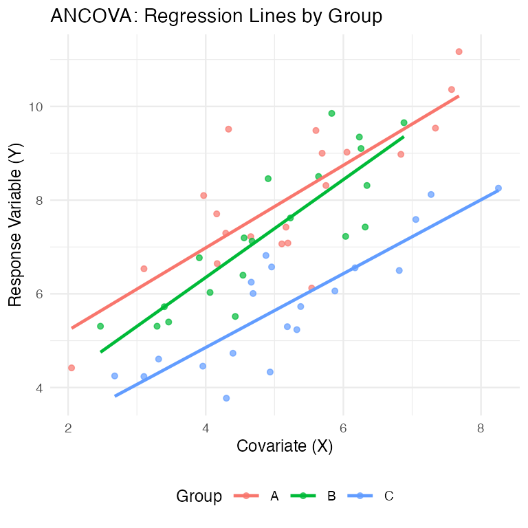
ANCOVA = Analysis of COVAriance — regression and ANOVA in one model. You use it when you have:

• a continuous response (Y)
• a categorical predictor (factor A)
• a continuous predictor, the covariate (X)

Two things it is for:

1. Compare group means after adjusting for the covariate
2. Ask whether two or more regression lines differ — in slope, in intercept, or both

When to Use ANCOVA

• Common Applications of ANCOVA
  • Increasing statistical power

    • The covariate (e.g., body size, initial temperature) explains some of the “noise” (residual error) in the response variable.

    • By “removing” this variation, we reduce the residual error, making it easier to detect the true effect of our categorical factor.

    • This results in a more powerful test of treatment effects.

  • Adjusting for confounding variables

    • Imagine your treatment groups happen to differ in their average covariate value (e.g., Group A was tested in a warmer room than Group B).

    • ANCOVA allows you to separate the treatment effect from the covariate effect.

  • Testing equality of regression lines
    • Do treatments have the same relationship (slope) with a continuous variable?

The Motivating Problem — Grayling in Two Lakes

Back to the Arctic grayling from week 5 — the same fish, a new question.

Lake I8 fish weigh more than lake I3 fish. But I8 fish are also longer (mean 364 mm vs 266 mm).

Is there a lake effect on mass at all, or are I8 fish simply bigger?

You cannot answer that by comparing mean masses. The groups differ in the very thing that drives the response.

Two Problems, One Tool

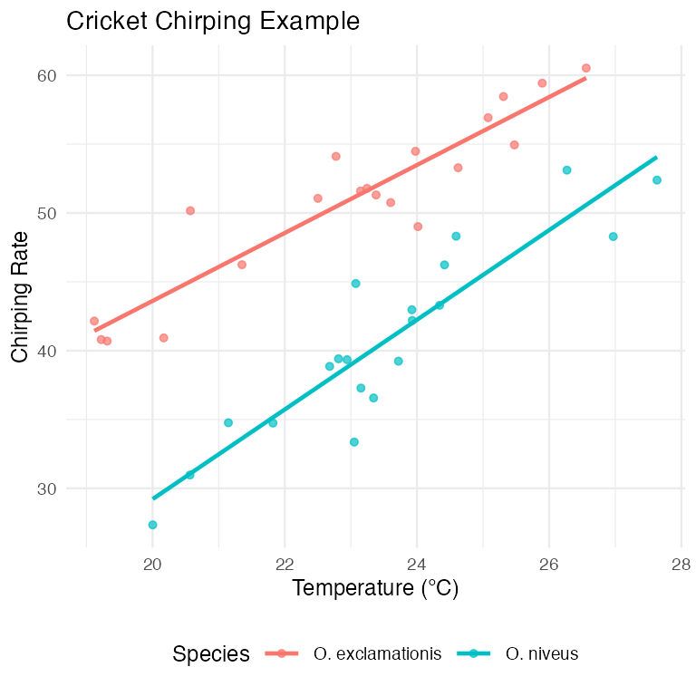
Problem 1 — confounding. The groups differ in the covariate, so a raw comparison of means confuses the treatment with the covariate. This is the grayling problem, and the classic cricket problem (two species measured at different temperatures).

Problem 2 — noise. Even when the groups are balanced on the covariate, the covariate still soaks up residual variation. Removing it shrinks the error term and makes the test of the factor more powerful. This is the fruitfly problem in Part 4.

Important

ANCOVA does both with one model

\[y \sim \underbrace{x}_{\text{covariate}} + \underbrace{A}_{\text{factor}}\]

It compares groups at a common value of the covariate — the “level playing field” comparison — instead of wherever each group happened to sit.

Warning

⚠️ One rule before you start

The covariate must be measured independently of the treatment, and must not be affected by it. Adjusting for something the treatment caused removes the very effect you are trying to measure.

Part 2 · The ANCOVA Model

ANCOVA Linear Model: Conceptual Framework

• The ANCOVA Model
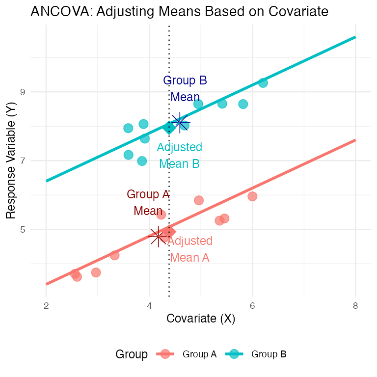
  • Key concept: Dfference between “unadjusted” group means and “adjusted” means
• In this visualization:
  • Group Means (asterisks): The raw average X and Y for each group.
  • Group A and Group B have different mean X values. Comparing directly misleading
  • Adjusted Means (triangles): ANCOVA statistically “moves” each group mean along regression line to single, common X value (the overall mean X).
  • ANCOVA compares heights (the Y values) of adjusted means.
  • Adjustment “levels the playing field,” estimating each group’s mean if all groups had same average covariate value

ANCOVA Model Visualization

Mathematical Model for ANCOVA

• Single-factor ANCOVA with
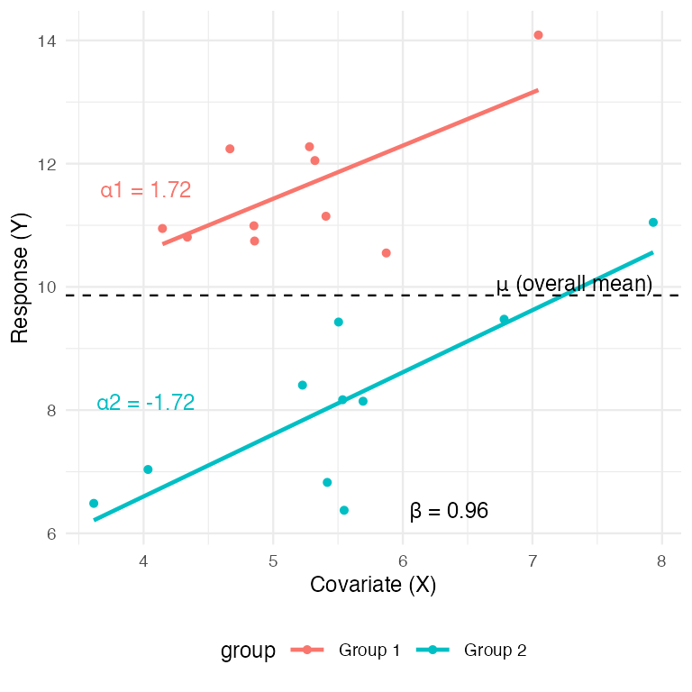
  • factor A (p levels, i = 1 to p), a continuous covariate (x), and response variable (y): \(Y_{ij} = \mu + \alpha_i + \beta(X_{ij} - \bar{X}) + \varepsilon_{ij}\)
• Where:
  • \(Y_{ij}\) = response value for observation j in level i of factor A
  • \(\mu\) = overall mean
  • \(\alpha_i\) = effect of level i of factor A (what we test in ANOVA)
  • \(\beta\) = common regression slope relating Y to X (what we test in Regression)
  • \(X_{ij}\) = covariate value for observation j in level i of factor A
  • \(\bar{X}\) = mean value of covariate
  • \(\varepsilon_{ij}\) = error term

ANCOVA Parameters Interpretation

• Interpretation of Parameters
  • \(\mu\) = overall mean response
  • \(\alpha_i\) = effect of level i (difference between group’s adjusted mean and overall mean)
  • \(\beta\) = pooled within-group regression coefficient (the slope)
  • \(X_{ij}\) = covariate value for observation j in group i
  • \(\bar{X}\) = overall mean of covariate
  • \(\varepsilon_{ij}\) = unexplained error
• Model assumes homogeneous slopes (i.e., \(\beta\) same for all groups) .

Building the ANCOVA Model in R

• Remember lm(y ~ predictor).
  • ANCOVA combines the predictors from ANOVA and regression.
• Simple Linear Regression:
  • Predict y using a continuous variable x.
    • model_reg <- lm(y ~ x, data = mydata)
• One-Way ANOVA:
  • We want to compare y among groups in a categorical factor A.
    • model_aov <- lm(y ~ A, data = mydata)
• ANCOVA (Additive Model):
  • Compare y among groups in A, after accounting for effect of x.
  • Add terms together
    • model_ancova <- lm(y ~ A + x, data = mydata)
  • Model assumes slope of y ~ x relationship is same for all groups in A.

Building the ANCOVA Model in R — The Two Formulas

• ANCOVA (Interaction Model):
  • What if the slopes are different for each group?
  • Test for interaction between factor and covariate.
    • model_int <- lm(y ~ A * x, data = mydata)
  • Shorthand for: lm(y ~ A + x + A:x, data = mydata)
  • The A:x term tests if the slopes are different.

ANCOVA in R: Workflow Steps 1 and 2

• Step 1: Test for Homogeneity of Slopes - Always Start Here

  • Fit interaction model first - tests key assumption that all groups share same slope.

  # The asterisk * tests for both main effects AND the interaction
  model_int <- lm(y ~ A * x, data = mydata)

• Step 2: Examine the Interaction Term

  • ANOVA table for model_int and find the p-value for interaction term (A:x).

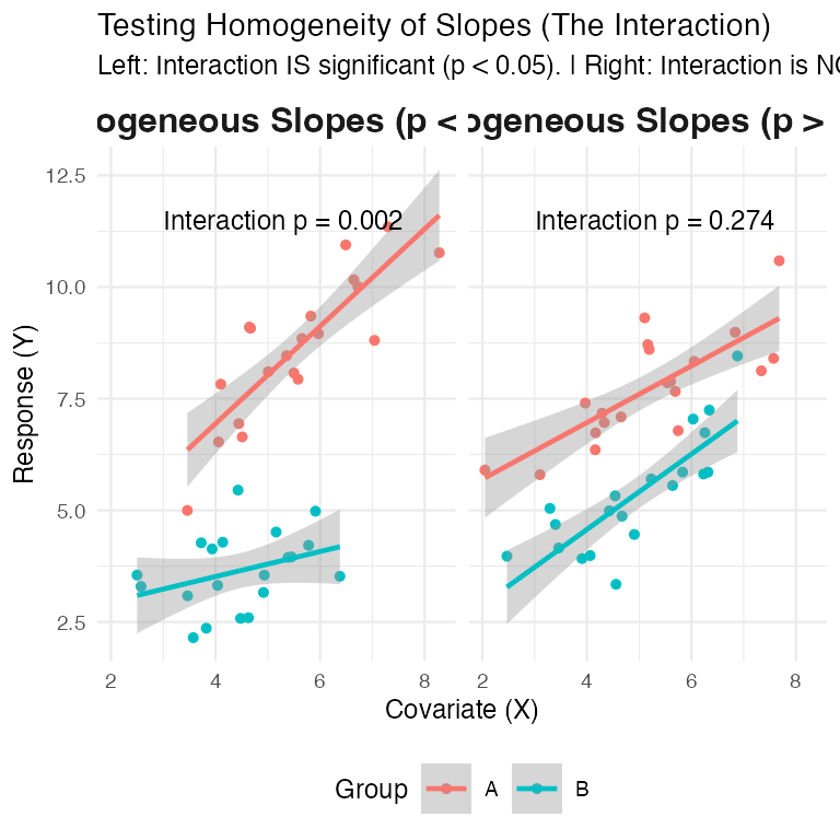
      Anova(model_int, type = "III")

  • If p > 0.05 (e.g., p = 0.4) - interaction IS NOT significant - slopes are homogeneous (parallel).
  • If p < 0.05 (e.g., p = 0.02): - interaction IS significant - slopes heterogeneous (NOT parallel).
  • ** standard ANCOVA model (y ~ A + x) inappropriate**
  • Analysis stops here and interpret interaction (often most interesting result!)

ANCOVA in R: Workflow Step 3

• Step 3: Run the ANCOVA (Additive Model)

  • If interaction not significant, run the simpler additive model the final ANCOVA model.

  # We use the + sign, which means "additive"
  model_ancova <- lm(y ~ A + x, data = mydata)
  # Get the final ANCOVA table
  Anova(model_ancova, type = "III")
  # Get the adjusted means
  library(emmeans)
  emmeans(model_ancova, "A")

Part 3 · Partitioning Variance & the ANOVA Table

Analysis of Variance for ANCOVA: Partitioning

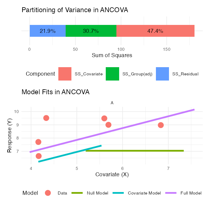
ANOVA Table for ANCOVA

The ANOVA table for a single-factor ANCOVA has these components:

# Create a tibble with ANOVA table information
anova_table <- tibble(
  Source = c("Factor A (adjusted)", "Covariate", "Residual", "Total"),
  df = c("(p-1)", "1", "n-p-1", "n-1"),
  `Sum of Squares` = c("SS_A(adj)", "SS_Covariate", "SS_Residual", "SS_Total"),
  `Mean Square` = c(
    "MS_A(adj) = SS_A(adj)/(p-1)",
    "MS_Covariate = SS_Covariate/1",
    "MS_Residual = SS_Residual/(n-p-1)",
    ""
  ),
  `F-ratio` = c("MS_A(adj)/MS_Residual", "MS_Covariate/MS_Residual", "", ""),
  `Expected MS` = c("σ² + n∑α²/(p-1)", "σ² + β²∑(X-X̄)²", "σ²", "")
)

# Create
anova_table
## # A tibble: 4 × 6
##   Source            df    `Sum of Squares` `Mean Square` `F-ratio` `Expected MS`
##   <chr>             <chr> <chr>            <chr>         <chr>     <chr>        
## 1 Factor A (adjust… (p-1) SS_A(adj)        "MS_A(adj) =… "MS_A(ad… "σ² + n∑α²/(…
## 2 Covariate         1     SS_Covariate     "MS_Covariat… "MS_Cova… "σ² + β²∑(X-…
## 3 Residual          n-p-1 SS_Residual      "MS_Residual… ""        "σ²"         
## 4 Total             n-1   SS_Total         ""            ""        ""

Null Hypotheses in ANCOVA

Homogeneity of Slopes (Test this first!)

\[H_0: \beta_1 = \beta_2 = ... = \beta_p\]

Are the regression slopes the same for all groups?

Test with the A:x interaction term in lm(y ~ A * x).

Important

This one is an assumption check, not a result. You want to fail to reject it before going any further.

Null Hypotheses in ANCOVA — the Two Results

Treatment effect, adjusted

\[H_0: \alpha_1 = \alpha_2 = \dots = \alpha_p = 0\]

Are the adjusted group means equal?

\[F = \frac{MS_{A(adj)}}{MS_{residual}}\]

the A term in lm(y ~ x + A).

Covariate effect

\[H_0: \beta = 0\]

Does the covariate relate to the response at all?

\[F = \frac{MS_{covariate}}{MS_{residual}}\]

the x term in lm(y ~ x + A).

Visualization of Homogeneity of Slopes

Parallel vs. Non-Parallel Slopes

Part 4 · Worked Example — Fruitfly Longevity

Partridge Example: Data Overview

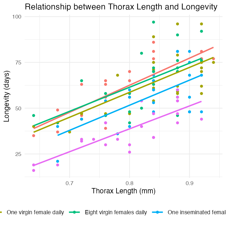
ANCOVA on Longevity of Male Fruitflies

Partridge Example: Steps 1–2 — Test Homogeneity of Slopes

homo_slopes_model <- lm(LONGEV ~ THORAX * treatment,
                        data = partridge)

Anova(homo_slopes_model, type = "III")
## Anova Table (Type III tests)
## 
## Response: LONGEV
##                   Sum Sq  Df  F value                Pr(>F)    
## (Intercept)       2963.8   1  26.0142           0.000001349 ***
## THORAX           12805.8   1 112.3988 < 0.00000000000000022 ***
## treatment           36.9   4   0.0810                0.9881    
## THORAX:treatment    42.5   4   0.0933                0.9844    
## Residuals        13102.1 115                                   
## ---
## Signif. codes:  0 '***' 0.001 '**' 0.01 '*' 0.05 '.' 0.1 ' ' 1

The interaction THORAX:treatment has p = 0.984 — about as far from significant as it gets.

The five treatment groups share a common slope: body size buys the same amount of extra life in every group.

Note

✅ Proceed to Step 3. Drop the interaction and fit the additive model.

Partridge Example: Step 3 — Fit the Additive ANCOVA

• Since the interaction was not significant, we re-run the model without it.
  • Interpretation:
    • THORAX: covariate highly significant
    • thorax length explains significant amount of variance in longevity
    • treatment: treatment effect, after adjusting for thorax length, is highly significant

# Step 3: Fit the ANCOVA model (additive model)
ancova_model <- lm(LONGEV ~ THORAX + treatment, data = partridge)
# View the final ANCOVA table
Anova(ancova_model, type = "III")
## Anova Table (Type III tests)
## 
## Response: LONGEV
##              Sum Sq  Df F value                Pr(>F)    
## (Intercept)  3069.7   1  27.791    0.0000006122893158 ***
## THORAX      13168.9   1 119.219 < 0.00000000000000022 ***
## treatment    9611.5   4  21.753    0.0000000000001719 ***
## Residuals   13144.7 119                                  
## ---
## Signif. codes:  0 '***' 0.001 '**' 0.01 '*' 0.05 '.' 0.1 ' ' 1

What the Covariate Bought You

Run the same question without the covariate, and compare:

# one-way ANOVA, covariate ignored
Anova(lm(LONGEV ~ treatment, data = partridge),
      type = 2)
## Anova Table (Type II tests)
## 
## Response: LONGEV
##           Sum Sq  Df F value         Pr(>F)    
## treatment  11939   4  13.612 0.000000003516 ***
## Residuals  26314 120                           
## ---
## Signif. codes:  0 '***' 0.001 '**' 0.01 '*' 0.05 '.' 0.1 ' ' 1

# ANCOVA, thorax length included
Anova(lm(LONGEV ~ THORAX + treatment, data = partridge),
      type = 2)
## Anova Table (Type II tests)
## 
## Response: LONGEV
##            Sum Sq  Df F value                Pr(>F)    
## THORAX    13168.9   1 119.219 < 0.00000000000000022 ***
## treatment  9611.5   4  21.753    0.0000000000001719 ***
## Residuals 13144.7 119                                  
## ---
## Signif. codes:  0 '***' 0.001 '**' 0.01 '*' 0.05 '.' 0.1 ' ' 1

	one-way ANOVA	ANCOVA
residual SS	26,314	13,145
residual df	120	119
treatment F	13.61	21.75

Important

Thorax length absorbed half the residual variation.

One degree of freedom spent on the covariate cut the error term from 26,314 to 13,145, and the test of treatment got 60% bigger (F 13.6 → 21.8) — on identical data and an identical question.

That is the power argument, and it is why you measure a covariate even when your groups are perfectly balanced on it.

Here the treatment effect was significant either way. On a smaller or noisier dataset, that difference is the difference between finding the effect and missing it.

Partridge Example: Getting Adjusted Means

• The ANOVA table tells us the treatments are different, but not which ones.

  • Use emmeans package to get the adjusted means / perform pairwise comparisons

  • The “estimated marginal mean” (or adjusted mean)

  • predicted longevity for each group, assuming an average thorax length

  • This is the “level playing field” comparison.

# Get adjusted means using emmeans
library(emmeans)
adjusted_means <- emmeans(ancova_model, "treatment")
adjusted_means
##  treatment                       emmean   SE  df lower.CL upper.CL
##  No females                        61.5 2.11 119     57.3     65.7
##  One inseminated female daily      64.2 2.10 119     60.0     68.3
##  Eight inseminated females daily   65.4 2.11 119     61.3     69.6
##  One virgin female daily           54.5 2.11 119     50.3     58.7
##  Eight virgin females daily        41.6 2.12 119     37.4     45.8
## 
## Confidence level used: 0.95

Partridge Example: Pairwise Comparisons

pairs(adjusted_means, adjust = "tukey")
##  contrast                                                       estimate   SE
##  No females - One inseminated female daily                         -2.65 2.98
##  No females - Eight inseminated females daily                      -3.93 3.00
##  No females - One virgin female daily                               7.02 2.97
##  No females - Eight virgin females daily                           19.95 3.01
##  One inseminated female daily - Eight inseminated females daily    -1.28 2.98
##  One inseminated female daily - One virgin female daily             9.67 2.98
##  One inseminated female daily - Eight virgin females daily         22.60 2.99
##  Eight inseminated females daily - One virgin female daily         10.95 3.00
##  Eight inseminated females daily - Eight virgin females daily      23.88 2.97
##  One virgin female daily - Eight virgin females daily              12.93 3.01
##   df t.ratio p.value
##  119  -0.891  0.8996
##  119  -1.311  0.6849
##  119   2.361  0.1336
##  119   6.636 <0.0001
##  119  -0.428  0.9929
##  119   3.249  0.0129
##  119   7.560 <0.0001
##  119   3.650  0.0035
##  119   8.031 <0.0001
##  119   4.298  0.0003
## 
## P value adjustment: tukey method for comparing a family of 5 estimates

Six of the ten are significant. The four that are not:

• No females vs. one inseminated — p = 0.90
• No females vs. eight inseminated — p = 0.68
• One vs. eight inseminated — p = 0.99
• No females vs. one virgin — p = 0.13

Every group that actually mated differs from the groups that did not, except the single-virgin group — the mildest treatment.

Partridge Example: Pairwise Comparisons — Compact Letters

##  treatment                       emmean   SE  df lower.CL upper.CL .group
##  Eight virgin females daily        41.6 2.12 119     37.4     45.8  a    
##  One virgin female daily           54.5 2.11 119     50.3     58.7   b   
##  No females                        61.5 2.11 119     57.3     65.7   bc  
##  One inseminated female daily      64.2 2.10 119     60.0     68.3    c  
##  Eight inseminated females daily   65.4 2.11 119     61.3     69.6    c  
## 
## Confidence level used: 0.95 
## P value adjustment: tukey method for comparing a family of 5 estimates 
## significance level used: alpha = 0.05 
## NOTE: If two or more means share the same grouping symbol,
##       then we cannot show them to be different.
##       But we also did not show them to be the same.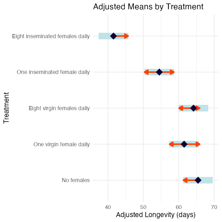

Groups sharing a letter are not distinguishable. The red arrows say the same thing — overlapping arrows mean no significant difference.

Important

Read the pattern, not the ranking

The three non-mating groups are one block. One virgin female pulls longevity down a little; eight pulls it down a lot.

The dose that matters is matings, not company.

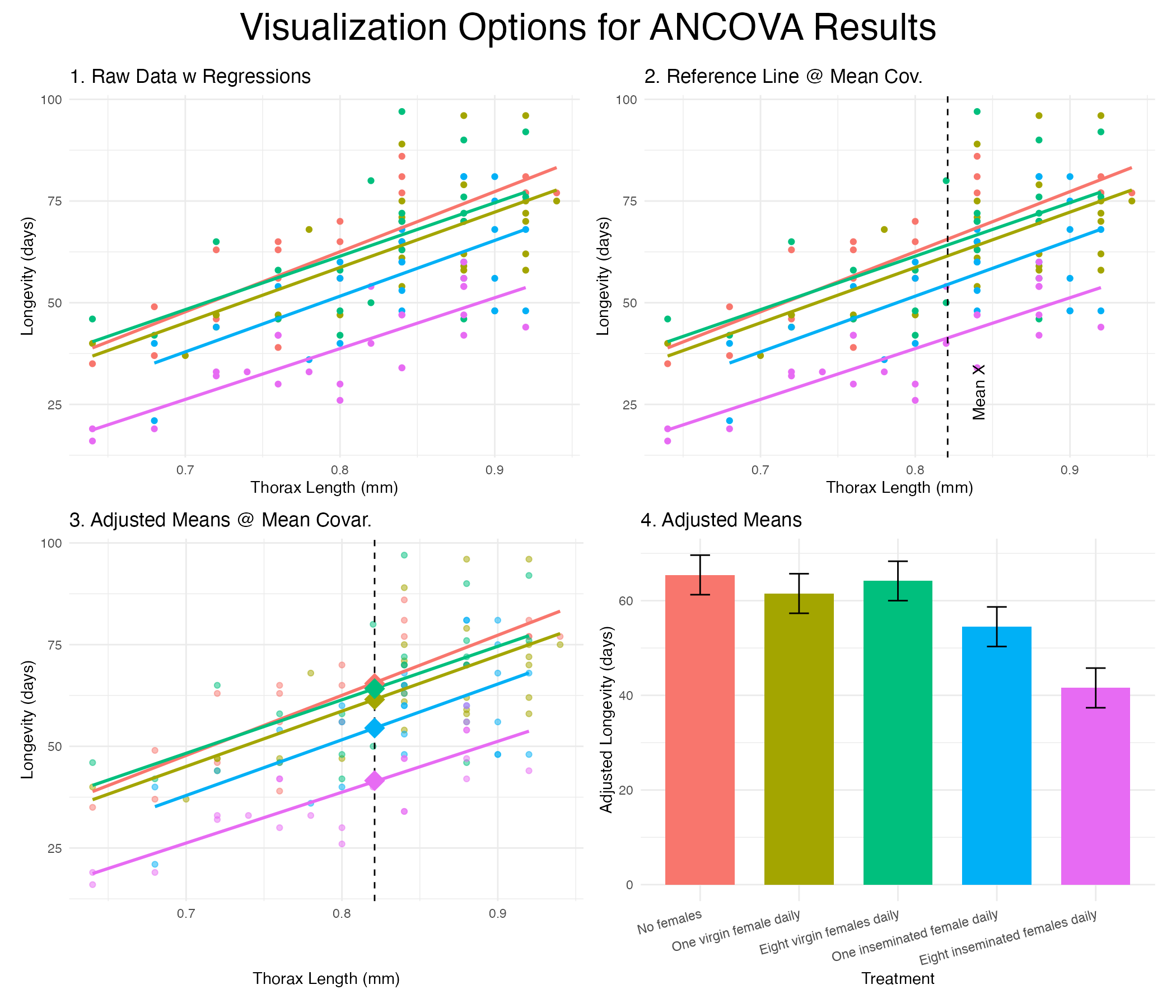
Visualizing ANCOVA Results

Visualization Options for ANCOVA

A 2x2 panel comparing four ways to visualize ANCOVA results for the fruitfly data: raw data with regression lines by treatment, the same plot with a reference line at the mean covariate, adjusted means plotted as diamonds at the mean covariate, and a bar chart of adjusted means with confidence-interval error bars.

Part 5 · Heterogeneous Slopes & Assumptions

What if the Slopes Are HETEROGENEOUS?

Back to the grayling. Fit the interaction model first, as always:

g_int <- lm(log_mass ~ log_len * lake, data = g_df)

Anova(g_int, type = 3)
## Anova Table (Type III tests)
## 
## Response: log_mass
##              Sum Sq  Df   F value                Pr(>F)    
## (Intercept)  1.8929   1 1337.5062 < 0.00000000000000022 ***
## log_len      4.0602   1 2868.9446 < 0.00000000000000022 ***
## lake         0.0094   1    6.6452              0.010833 *  
## log_len:lake 0.0117   1    8.2518              0.004617 ** 
## Residuals    0.2293 162                                    
## ---
## Signif. codes:  0 '***' 0.001 '**' 0.01 '*' 0.05 '.' 0.1 ' ' 1

The interaction is significant (p = 0.0046). The two lakes do not share a slope.

Important

Stop. Do not fit the additive model.

log_mass ~ log_len + lake would force one common slope through two populations that do not have one, and then report a single “lake effect” that is true at no particular length.

There is no such thing as the difference between the lakes here. The difference depends on how big the fish is.

Note

📖 This is not a failure

A significant interaction is usually the more interesting result. It says the groups differ in how the response scales, not merely in where it sits.

Reading Heterogeneous Slopes — emtrends()

emtrends(g_int, "lake", var = "log_len")
##  lake log_len.trend     SE  df lower.CL upper.CL
##  I3            2.79 0.0943 162     2.61     2.98
##  I8            3.11 0.0569 162     3.00     3.22
## 
## Confidence level used: 0.95

pairs(emtrends(g_int, "lake", var = "log_len"))
##  contrast estimate   SE  df t.ratio p.value
##  I3 - I8    -0.316 0.11 162  -2.873  0.0046

emtrends() is emmeans() for slopes. It gives one slope per group, with a standard error, and pairs() tests whether they differ.

On log-log axes the slope is the allometric exponent: mass ∝ length^b.

Important

The biology is in the exponent

• I8: b = 3.11 — not distinguishable from 3 (p = 0.058). Isometric: these fish keep their shape as they grow.
• I3: b = 2.79 — significantly below 3 (p = 0.029). I3 grayling get relatively lighter as they lengthen.

That is a condition difference between the lakes, and an additive ANCOVA would have hidden it entirely.

Where Do the Groups Actually Differ?

With non-parallel lines, the gap between groups changes along the covariate. So ask for the contrast at specific covariate values:

lens <- log10(c(200, 250, 300))

pairs(emmeans(g_int, ~ lake | log_len,
              at = list(log_len = lens)))
## log_len = 2.30:
##  contrast estimate      SE  df t.ratio p.value
##  I3 - I8   -0.0299 0.01940 162  -1.540  0.1256
## 
## log_len = 2.40:
##  contrast estimate      SE  df t.ratio p.value
##  I3 - I8   -0.0605 0.01110 162  -5.479 <0.0001
## 
## log_len = 2.48:
##  contrast estimate      SE  df t.ratio p.value
##  I3 - I8   -0.0856 0.00914 162  -9.370 <0.0001

Length	I3 − I8 (log mass)	p
200 mm	−0.030	0.13
250 mm	−0.061	<0.0001
300 mm	−0.107	<0.0001

At 200 mm the two lakes are indistinguishable. The gap opens as the fish get longer, and by 300 mm an I3 grayling is about 20% lighter than an I8 grayling of the same length.

Warning

⚠️ johnson_neyman = TRUE does not work here

The Johnson–Neyman procedure needs a continuous moderator. interactions::sim_slopes() will warn “Johnson-Neyman intervals are not available for factor predictors or moderators” and give you nothing. With a categorical factor, the contrast-at-covariate-values above is the right tool.

Handling Heterogeneous Slopes — the Options

When the interaction is significant:

1. Report the interaction. It is the result. Give the slopes, not an adjusted mean.
2. emtrends() for a slope per group, with pairs() to test them.
3. Contrast at chosen covariate values — emmeans(~ A | x, at = ...) — to say where along the covariate the groups separate.
4. Johnson–Neyman, but only when the moderator is continuous.
5. Separate regressions per group. Simple, honest, least powerful, and it gives up the shared error term.

Warning

⚠️ Mind the covariate ranges

I3 fish run 191–320 mm; I8 fish run 207–440 mm. The lines can only be compared where both groups have data.

Reporting a lake difference at 400 mm would mean extrapolating the I3 line past every I3 fish ever measured. ANCOVA will do that arithmetic without complaint. You have to be the one who refuses.

Note

This caution applies to the additive model too — an “adjusted mean” at \(\bar{x}\) is an extrapolation for any group whose data does not reach \(\bar{x}\).

Assumptions of ANCOVA

#	Assumption	How you check it
1	Independence	design, not a test
2	Normal residuals	Q-Q plot
3	Equal variances	residuals vs. fitted
4	Linearity of Y on X within each group	scatterplot
5	Homogeneity of slopes	the A:x interaction

Important

#5 is the one that is special to ANCOVA, and the only one you test before fitting the model you will report. The other four are the ordinary linear-model assumptions you have been checking since week 7.

Warning

⚠️ And one that is not on the list

The covariate must be independent of the treatment. No test will catch a violation — only knowing how the data were collected will.

Checking Assumptions in R

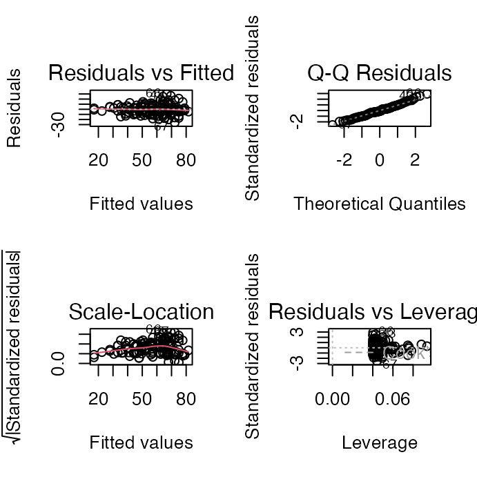
Check assumptions 2 and 3 on the final model — the additive one, if the slopes let you fit it.

• Residuals vs. fitted — red line roughly flat at 0 ✅
• Normal Q-Q — points on the dashed line ✅
• Scale-location — red line flat ✅
• Residuals vs. leverage — nothing stranded in the right-hand corners ✅

Note

Conclusion: the assumptions are met, so the ANCOVA table on the previous slides can be reported as it stands.

Robust ANCOVA Approaches

When the assumptions are badly violated — not marginally:

• Rank transformation — rank both Y and X, then run the ordinary ANCOVA on the ranks: lm(rank(y) ~ rank(x) + A)
• Bootstrapping — resample to get intervals without assuming normality
• Quantile regression — model the median, or any quantile, instead of the mean
• Permutation tests — randomise the treatment labels to build the null distribution

Tip

🖐 Run it as a sensitivity check. If the robust version agrees with the parametric one, report the parametric one and say you checked.

rank_ancova <- lm(rank(LONGEV) ~ rank(THORAX) + treatment,
                  data = partridge)

signif(c(
  parametric = Anova(ancova_model, type = "III")["treatment", "Pr(>F)"],
  rank_based = Anova(rank_ancova,  type = "III")["treatment", "Pr(>F)"]), 3)
##        parametric        rank_based 
## 0.000000000000172 0.000000000000654

Both vanishingly small — the parametric result stands.

Part 6 · Reporting Results

Writing Up ANCOVA Results

Scientific Writing Example

Here’s how you might write up ANCOVA results for publication:

“We analyzed the effects of mating opportunity on male fruitfly longevity using analysis of covariance (ANCOVA), with thorax length as a covariate. Before conducting the main analysis, we tested the homogeneity-of-slopes assumption and found no significant treatment × thorax length interaction (F₄,₁₁₅ = 0.09, P = 0.98), indicating that the effect of body size on longevity was consistent across treatments.

The ANCOVA revealed significant effects of both treatment (F₄,₁₁₉ = 21.75, P < 0.001) and thorax length (F₁,₁₁₉ = 119.22, P < 0.001) on longevity. Thorax length was positively associated with longevity.

After adjusting for body size, longevity declined with the number of virgin females a male was housed with (adjusted mean ± SE: 54.5 ± 2.11 days for one virgin female and 41.6 ± 2.12 days for eight, versus 61.5 ± 2.11 days for males housed alone). Males housed with inseminated females — which do not mate — did not differ from males housed alone (64.2 ± 2.10 and 65.4 ± 2.11 days; Tukey P = 0.90 and P = 0.68). Six of the ten pairwise comparisons were significant at P < 0.05; the four that were not were the three comparisons among the non-mating groups and the no-females vs. one-virgin-female comparison (P = 0.13).”

Why the Inseminated-Female Groups Are the Design

Important

The control that makes the experiment work

Newly inseminated females will not mate. Males housed with them get the presence of females without the mating.

Those groups isolate the cost of mating itself from the cost of simply having company — and they show no reduction in longevity at all (65.4 and 64.2 days, against 61.5 for males housed alone).

Note

📖 What this buys the write-up

Without those two groups you could only say “males near females die younger,” which has at least three explanations. With them, the conclusion narrows to one.

Design, not statistics, is what rules out the alternatives. ANCOVA just made the comparison fair on body size.

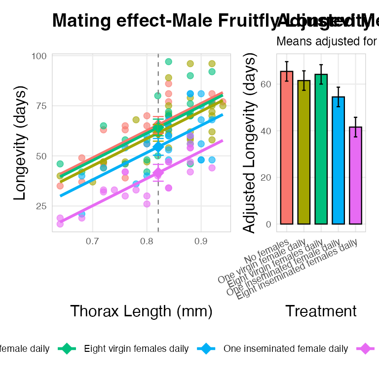
Publication Quality Figure

Summary

What it is for

• Combines regression and ANOVA
• Increases power by soaking up residual variation with a covariate
• Adjusts for confounds by comparing groups at a common covariate value

The workflow

1. Always test homogeneity of slopes first — lm(y ~ A * x)
2. Slopes homogeneous (p > 0.05) → fit the additive model, lm(y ~ x + A), and report adjusted means
3. Slopes heterogeneous (p < 0.05) → stop. Interpret the interaction and report slopes

Summary — Interpreting and Reporting

Interpretation

• car::Anova(model, type = "III") for the table
• emmeans() for adjusted means and pairwise comparisons
• emtrends() for slopes, when the interaction is the result
• Report adjusted means, and say what covariate value they are adjusted to

The five assumptions

1. Independence
2. Normal residuals
3. Equal variances
4. Linearity within groups
5. Homogeneity of slopes — the one you test first

Important

And the one no test will find: the covariate must not be affected by the treatment.

Readings

• Quinn & Keough (2002), Experimental Design and Data Analysis for Biologists, Ch. 12 — Analysis of Covariance. This is the source of today’s fruitfly example (Box 12-1, Table 12-2).
• Gotelli & Ellison, Ch. 9 (Regression) and Ch. 10 (The Analysis of Variance) — ANCOVA sits across the two frameworks.
• Whitlock & Schluter, Ch. 17 — Regression, for the diagnostics that carry over.
• Partridge, L., & Farquhar, M. (1981). Sexual activity reduces lifespan of male fruitflies. Nature, 294, 580–582.

Note

📖 On the datasets

The fruitfly data are Partridge & Farquhar’s, reproduced in Quinn & Keough Box 12-1. The Arctic grayling are from the Arctic LTER — the same lakes you met in week 5.

The textbook PDFs are on Canvas.

Tip

🖐 The homework crickets

Walker’s (1962) cricket data is Homework 10. It is the same shape of question as the grayling — two groups, one covariate — and you decide for yourself whether the slopes let you fit an additive model.