Lecture: Two-Way ANOVA

Factorial designs

Factorial (two-factor) ANOVA, main effects and interactions, estimated marginal means, Type I/II/III sums of squares, and balanced vs. unbalanced designs — on the palmerpenguins species-by-sex dataset.

Where We Left Off

Covered last time — one-way ANOVA:

• Analysis of variance: single and multi-factor designs
• Examples: diatoms, circadian rhythms
• Predictor variables: fixed vs. random
• The ANOVA model
• Analysis and partitioning of variance
• Null hypothesis
• Assumptions and diagnostics
• Post-hoc F-tests — Tukey and others
• Reporting the results

Note

✅ Key idea from last lecture

One-way ANOVA asks “do these groups differ?” for one factor. Today: what happens when two factors act together — separately, and possibly interacting?

XKCD comic listing p-value ranges with increasingly tongue-in-cheek interpretations, from ‘Highly Significant’ at p under 0.03 down through ‘On the edge of significance’ and ‘Hey, look at this interesting subgroup analysis’ at p >= 0.1, captioned ‘If all else fails, use significant at a p>0.05 level and hope no one notices’ — a joke about p-hacking and misusing significance thresholds.

Part 1 · Factorial ANOVA — the Concept

Two-Factor Designs (2-Way ANOVA)

• Very common in ecology
• Can have more factors (e.g., 3-way ANOVA), but interpretation gets very challenging
• Most multifactor designs are factorial or nested
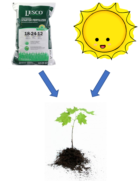
• We’ll cover a 2-factor ANOVA — this could be fertilizer and sunlight for plant biomass produced:
  • each can have an effect independently
  • the effect of one factor may interact with the other factor
  • example: a low- vs. high-light treatment might affect biomass; fertilizer might also affect biomass; but under higher light, the high-fertilizer treatment may grow better than expected

Note

📖 Reference

Gotelli & Ellison, A Primer of Ecological Statistics, Ch. 10 — The Analysis of Variance, extends to factorial designs like the one covered today.

Diagram of a fertilizer bag and a smiling sun icon, each with an arrow pointing down to a small green seedling, illustrating fertilizer and sunlight as two separate factors that can each affect plant biomass.

The palmerpenguins R package hex-sticker logo, showing simple cartoon illustrations of the three penguin species (Adelie, Chinstrap, Gentoo) used in this lecture’s dataset.

Factorial ANOVA: Design Structure

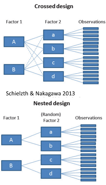
Consider two factors:

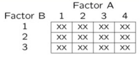
• Factorial/crossed: every level of B in every level of A

Cartoon illustration of the three penguin species used in this lecture’s dataset, each labeled: Chinstrap, Gentoo, and Adelie.

Diagram contrasting a crossed design, where both levels of Factor 1 (A, B) connect to every level of Factor 2 (a, b, c, d), against a nested design below it, where each level of Factor 1 connects only to its own subset of (random) Factor 2 levels, both feeding into individual observations (Schielzth & Nakagawa 2013).

Factorial ANOVA: Effect Types

In factorial designs, we look at two types of factor effects:

• Main effect of each factor (pooling across the other factor)
• Interaction effects — is there a synergistic/antagonistic effect between factors?

Simple grid diagram of a factorial design with Factor A across the columns (levels 1-4) and Factor B down the rows (levels 1-3), with an ‘XX’ marking every cell, showing every combination of the two factors is represented.

Part 2 · Setting Up — the Penguin Data

Introduction to Two-Way ANOVA

Two-way ANOVA examines:

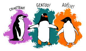
• Main effect of Factor A (Species)
• Main effect of Factor B (Sex)
• Interaction between A × B
• Balanced design: equal sample sizes in all cells
• Type III sums of squares for unbiased estimates — if the design is balanced, the choice of SS type doesn’t matter

## # A tibble: 6 × 6
##   species   sex        n mean_mass sd_mass se_mass
##   <fct>     <fct>  <int>     <dbl>   <dbl>   <dbl>
## 1 Adelie    female    73     3369.    269.    31.5
## 2 Adelie    male      73     4043.    347.    40.6
## 3 Chinstrap female    34     3527.    285.    48.9
## 4 Chinstrap male      34     3939.    362.    62.1
## 5 Gentoo    female    58     4680.    282.    37.0
## 6 Gentoo    male      61     5485.    313.    40.1

Data Preparation — Creating a Balanced Design

The penguin data frame is unbalanced — there are unequal samples per cell.

## # A tibble: 3 × 3
##   species   female  male
##   <fct>      <int> <int>
## 1 Adelie        73    73
## 2 Chinstrap     34    34
## 3 Gentoo        58    61

## Minimum n = 34
## # A tibble: 3 × 3
##   species   female  male
##   <fct>      <int> <int>
## 1 Adelie        34    34
## 2 Chinstrap     34    34
## 3 Gentoo        34    34

Statistical model:

\[Y_{ijk} = \mu + \alpha_i + \beta_j + (\alpha\beta)_{ij} + \varepsilon_{ijk}\]

μ = grand mean, α_i = effect of species i, β_j = effect of sex j, (αβ)_ij = interaction effect, ε_ijk = random error.

Descriptive Statistics

## # A tibble: 6 × 6
##   species   sex        n mean_mass sd_mass se_mass
##   <fct>     <fct>  <int>     <dbl>   <dbl>   <dbl>
## 1 Adelie    female    34     3335.    260.    44.5
## 2 Adelie    male      34     4049.    318.    54.5
## 3 Chinstrap female    34     3527.    285.    48.9
## 4 Chinstrap male      34     3939.    362.    62.1
## 5 Gentoo    female    34     4681.    309.    53.0
## 6 Gentoo    male      34     5525     274.    47.0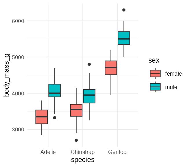

Part 3 · The Factorial Model

Factorial ANOVA Models

Factorial designs can be of 3 types:

• Model 1 — 2 fixed factors (the focus for today)
• Model 2 — 2 random factors
• Model 3 — 1 fixed, 1 random (mixed model) — often nested

Model 1 ANOVA:

\[y_{ijk} = \mu + \alpha_i + \beta_j + (\alpha\beta)_{ij} + \varepsilon_{ijk}\]

Tip

🖐 Notice

The formula looks identical to Model 2 and Model 3 — what changes between them is whether α, β are treated as fixed effects (specific groups you care about) or random effects (a sample from a larger population of possible groups).

Model Components — the Main Effects

\[y_{ijk} = \mu + \alpha_i + \beta_j + (\alpha\beta)_{ij} + \varepsilon_{ijk}\]

• \(y_{ijk}\): value of the k-th observation from the j-th and i-th combination of B and A (sex j of species i)
• μ: overall mean (overall mass)
• \(\alpha_i\): effect of the i-th level of A, pooling across all levels of B — \(\mu_i - \mu\) (difference between the average mass of all “species i” penguins and the overall mean)

Tip

🖐 Notice

Every effect in this model is defined as a deviation from a mean — the grand mean, or a group mean. This is exactly the same logic as a t-test or one-way ANOVA, just with more terms.

Model Components — the Interaction

\[y_{ijk} = \mu + \alpha_i + \beta_j + (\alpha\beta)_{ij} + \varepsilon_{ijk}\]

• \(\beta_j\): effect of the j-th level of B, pooling across all levels of A — \(\mu_j - \mu\) (difference between the average mass of all “sex j” penguins and the overall mean)
• \((\alpha\beta)_{ij}\): effect of the interaction of level i of A and level j of B — \(\mu_{ij} - \mu_i - \mu_j + \mu\). Does the effect of B depend on the level of A? (Is the effect of sex different across the 3 species?)

Note

✅ Key idea

The interaction term is what’s left over after you subtract out both main effects and the grand mean — it’s literally “the part the additive model can’t explain.”

Model Types and Interpretation

\[y_{ijk} = \mu + \alpha_i + \beta_j + (\alpha\beta)_{ij} + \varepsilon_{ijk}\]

• Model 2 ANOVA is rare in ecology
• Model 3 interpretation is different:
  • \(\beta_j\): random variable measuring variance in y across all possible levels of B, pooling across A
  • \((\alpha\beta)_{ij}\) is a random variable measuring variance of the interaction between A and B across all possible levels of B (“is the effect of A consistent across all possible levels of B that could have been chosen?”)

Warning

⚠️ Watch out!

Fixed vs. random isn’t about the data — it’s about the question. Are you interested in these specific 3 species (fixed), or in “species” as a general source of variation (random)?

Part 4 · Estimated Marginal Means

Estimated Marginal Means — Species

• Before we go further, we need to define estimated marginal means (EMMs)
• Balanced data: it’s just the means of the groups — easy
• Unbalanced data: it’s the mean of cell means, not a simple average of all raw observations

## Combined table with means and counts:
## # A tibble: 3 × 5
##   species   female_mean male_mean female_n male_n
##   <fct>           <dbl>     <dbl>    <int>  <int>
## 1 Adelie          3369.     4043.       73     73
## 2 Chinstrap       3527.     3939.       34     34
## 3 Gentoo          4680.     5485.       58     61
## 
## 
## Regular means (WRONG for marginal means):
## # A tibble: 3 × 3
##   species   total_n regular_mean
##   <fct>       <int>        <dbl>
## 1 Adelie        146        3706.
## 2 Chinstrap      68        3733.
## 3 Gentoo        119        5092.

## Estimated Marginal Means for Species (CORRECT):
## # A tibble: 3 × 3
##   species   emm_mean calculation                   
##   <fct>        <dbl> <chr>                         
## 1 Adelie       3706. (3368.8 + 4043.5) / 2 = 3706.2
## 2 Chinstrap    3733. (3527.2 + 3939) / 2 = 3733.1  
## 3 Gentoo       5082. (4679.7 + 5484.8) / 2 = 5082.3
## 
## 
## Comparison showing EMM calculation:
## # A tibble: 3 × 6
##   species   cell_mean_female cell_mean_male species_emm regular_mean difference
##   <fct>                <dbl>          <dbl>       <dbl>        <dbl>      <dbl>
## 1 Adelie               3369.          4043.       3706.        3706.   4.55e-13
## 2 Chinstrap            3527.          3939.       3733.        3733.   0       
## 3 Gentoo               4680.          5485.       5082.        5092.  -1.01e+ 1

Estimated Marginal Means — Sex

• Balanced data: just the means of the groups
• Unbalanced data: mean of cell means

## Combined table with means and counts:
## # A tibble: 3 × 5
##   species   female_mean male_mean female_n male_n
##   <fct>           <dbl>     <dbl>    <int>  <int>
## 1 Adelie          3369.     4043.       73     73
## 2 Chinstrap       3527.     3939.       34     34
## 3 Gentoo          4680.     5485.       58     61

## 
## Regular means sex (WRONG for marginal means):
## # A tibble: 2 × 3
##   sex    total_n regular_mean
##   <fct>    <int>        <dbl>
## 1 female     165        3862.
## 2 male       168        4546.
## 
## 
## Estimated Marginal Means for Sex (CORRECT):
## # A tibble: 2 × 3
##   sex    emm_mean calculation                            
##   <fct>     <dbl> <chr>                                  
## 1 female    3859. (3368.8 + 3527.2 + 4679.7) / 3 = 3858.6
## 2 male      4489. (4043.5 + 3939 + 5484.8) / 3 = 4489.1
## 
## 
## Comparison showing difference between regular and marginal means:
## # A tibble: 2 × 5
##   sex    total_n regular_mean emm_mean difference
##   <fct>    <int>        <dbl>    <dbl>      <dbl>
## 1 female     165        3862.    3859.      -3.68
## 2 male       168        4546.    4489.     -56.6

Part 5 · The Two-Way ANOVA Table

ANOVA Table Structure

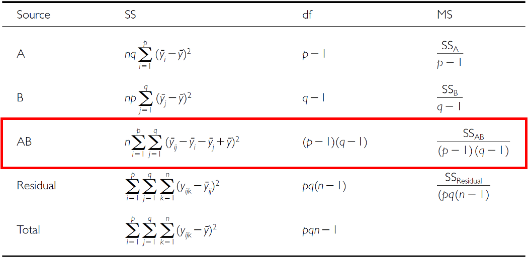
• \(SS_{total} = SS_A + SS_B + SS_{AB} + SS_{residual}\)
• \(SS_{total} = \sum(Y - \bar{Y})^2\)
• \(SS_{residual}\): the difference between each observation and its cell mean, summed over all observations

Source	df
A	p − 1
B	q − 1
AB	(p−1)(q−1)
Residual	pq(n−1)
Total	pqn − 1

where p = levels of A, q = levels of B, n = replicates per cell.

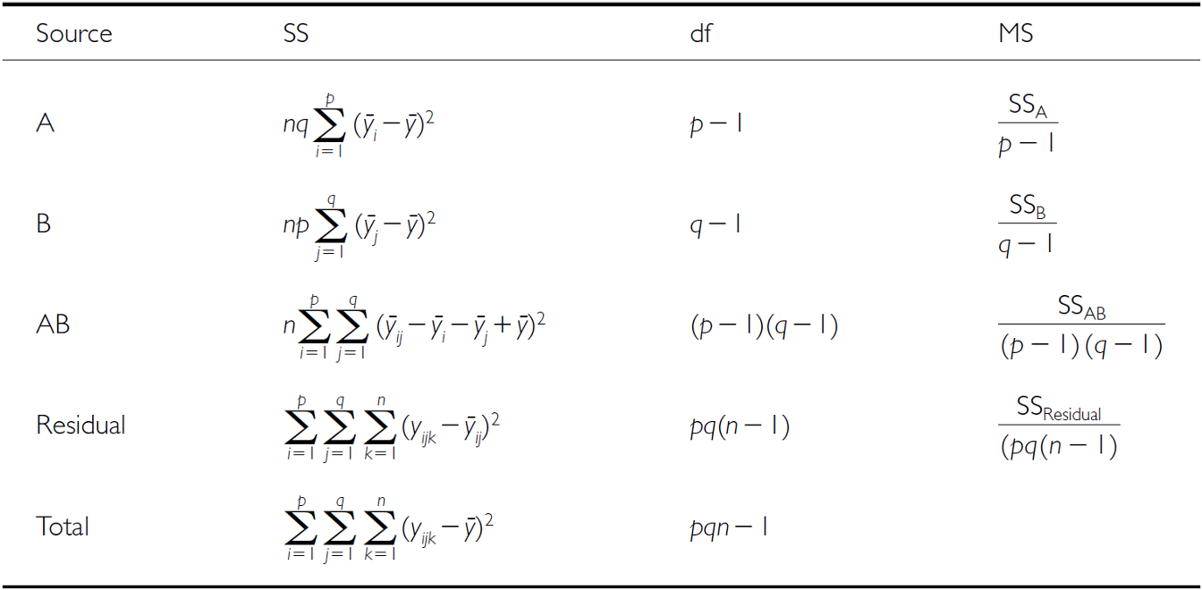
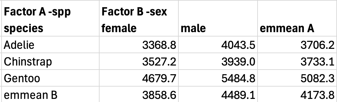
SSA: Factor A Effects

• \(SS_A\) is the SS of differences between each marginal mean of A and the overall mean
• If A is species, take the EMMs for factor A and subtract from the overall mean

Full two-way ANOVA table listing Source (A, B, AB, Residual, Total), each with its sum-of-squares formula, degrees of freedom (p-1, q-1, (p-1)(q-1), pq(n-1), pqn-1), and mean-square formula.

Table of penguin body mass cell means and marginal (emmean) values by species (rows: Adelie, Chinstrap, Gentoo) and sex (columns: female, male), used to compute SS_A from the species row means.

SSB: Factor B Effects

• \(SS_B\) is the SS of differences between each marginal mean of B and the overall mean
• If B is sex, take the EMMs for factor B and subtract from the overall mean

The same two-way ANOVA table (Source, SS, df, MS for A, B, AB, Residual, Total) repeated here for computing SS_B.

The same penguin body-mass cell-means and marginal-means table repeated here, used to compute SS_B from the sex column means.

SSAB: Interaction Effects

\(SS_{AB}\) is the SS of cell means minus marginal means plus the overall mean.

The same two-way ANOVA table with the AB (interaction) row outlined in red, highlighting its sum-of-squares, degrees of freedom (p-1)(q-1), and mean-square formulas.

The same penguin body-mass cell-means and marginal-means table repeated here, used to compute SS_AB from how each cell mean deviates from its row and column marginal means.

F-Ratio Calculations

SS converts to MS; F-ratio calculations differ depending on whether factors are fixed, random, or mixed.

Source	A, B fixed	A, B random	A fixed, B random
A	\(MS_A/MS_{Res}\)	\(MS_A/MS_{AB}\)	\(MS_A/MS_{AB}\)
B	\(MS_B/MS_{Res}\)	\(MS_B/MS_{AB}\)	\(MS_B/MS_{AB}\)
AB	\(MS_{AB}/MS_{Res}\)	\(MS_{AB}/MS_{Res}\)	\(MS_{AB}/MS_{Res}\)

Hypotheses — Both Factors Fixed

3 hypotheses are tested in a two-way factorial ANOVA: A, B, A×B. Both factors fixed:

• \(H_0(A)\): \(\mu_1 = \mu_2 = ... = \mu_p\) (no difference in marginal means of A, pooling across B)
• \(H_0(B)\): \(\mu_1 = \mu_2 = ... = \mu_q\) (no difference in marginal means of B, pooling across A)
• \(H_0(AB)\): \(\mu_{ij} - \mu_i - \mu_j + \mu = 0\) (no interaction effect)

Tip

🖐 Notice

These are exactly the two main-effect hypotheses from a one-way ANOVA, plus one new hypothesis just for the interaction.

Hypotheses — Mixed Model

3 hypotheses: A, B, A×B. One fixed, one random:

• \(H_0(A)\): \(\mu_1 = \mu_2 = ... = \mu_p\) (no difference in marginal means of A, pooling across B)
• \(H_0(B)\): \(\sigma^2_B = 0\) (no added variance due to levels of B that could have been used)
• \(H_0(AB)\): \(\sigma^2_{AB} = 0\) (no added variance due to interaction between all levels of A and B that could have been used)

Warning

⚠️ Watch out!

Notice the switch from “means are equal” (fixed) to “variance is zero” (random) — that’s the fundamental difference in what a random-effect hypothesis is even asking.

Part 6 · Fitting the Balanced Model

Example Study Details

Let’s try the example with the palmerpenguins package data:

• Effect of species and sex on body_mass_g
• 3 species (Factor A)
• 2 sexes (Factor B)
• 34 replicates in each cell

Cartoon illustration of the three penguin species used in this lecture’s dataset, each labeled: Chinstrap, Gentoo, and Adelie.

Two-Way ANOVA with Type III Sums of Squares

## 
## Call:
## lm(formula = body_mass_g ~ species * sex, data = balanced_df)
## 
## Residuals:
##     Min      1Q  Median      3Q     Max 
## -827.21 -178.13    6.25  175.00  861.03 
## 
## Coefficients:
##               Estimate Std. Error t value Pr(>|t|)    
## (Intercept)    4175.86      21.23 196.727  < 2e-16 ***
## species1       -484.31      30.02 -16.134  < 2e-16 ***
## species2       -442.77      30.02 -14.750  < 2e-16 ***
## sex1           -328.31      21.23 -15.467  < 2e-16 ***
## species1:sex1   -28.68      30.02  -0.955    0.341    
## species2:sex1   122.43      30.02   4.078 6.57e-05 ***
## ---
## Signif. codes:  0 '***' 0.001 '**' 0.01 '*' 0.05 '.' 0.1 ' ' 1
## 
## Residual standard error: 303.2 on 198 degrees of freedom
## Multiple R-squared:  0.8596, Adjusted R-squared:  0.856 
## F-statistic: 242.4 on 5 and 198 DF,  p-value: < 2.2e-16

## Type III Sums of Squares ANOVA:
## Anova Table (Type III tests)
## 
## Response: body_mass_g
##                 Sum Sq  Df    F value    Pr(>F)    
## (Intercept) 3557308900   1 38701.5271 < 2.2e-16 ***
## species       87725999   2   477.2049 < 2.2e-16 ***
## sex           21988483   1   239.2224 < 2.2e-16 ***
## species:sex    1672776   2     9.0994 0.0001657 ***
## Residuals     18199467 198                         
## ---
## Signif. codes:  0 '***' 0.001 '**' 0.01 '*' 0.05 '.' 0.1 ' ' 1

Understanding Type III SS

Type III sums of squares test each effect after adjusting for all other effects in the model:

• Species effect: tested after adjusting for sex and interaction
• Sex effect: tested after adjusting for species and interaction
• Interaction: tested after adjusting for both main effects

This is especially important for unbalanced designs, but we’re using it here for consistency with the next analysis.

## Effect Sizes (Eta-squared):
##        Effect Eta_Squared
## 1     Species  0.67696748
## 2         Sex  0.16968160
## 3 Interaction  0.01290854

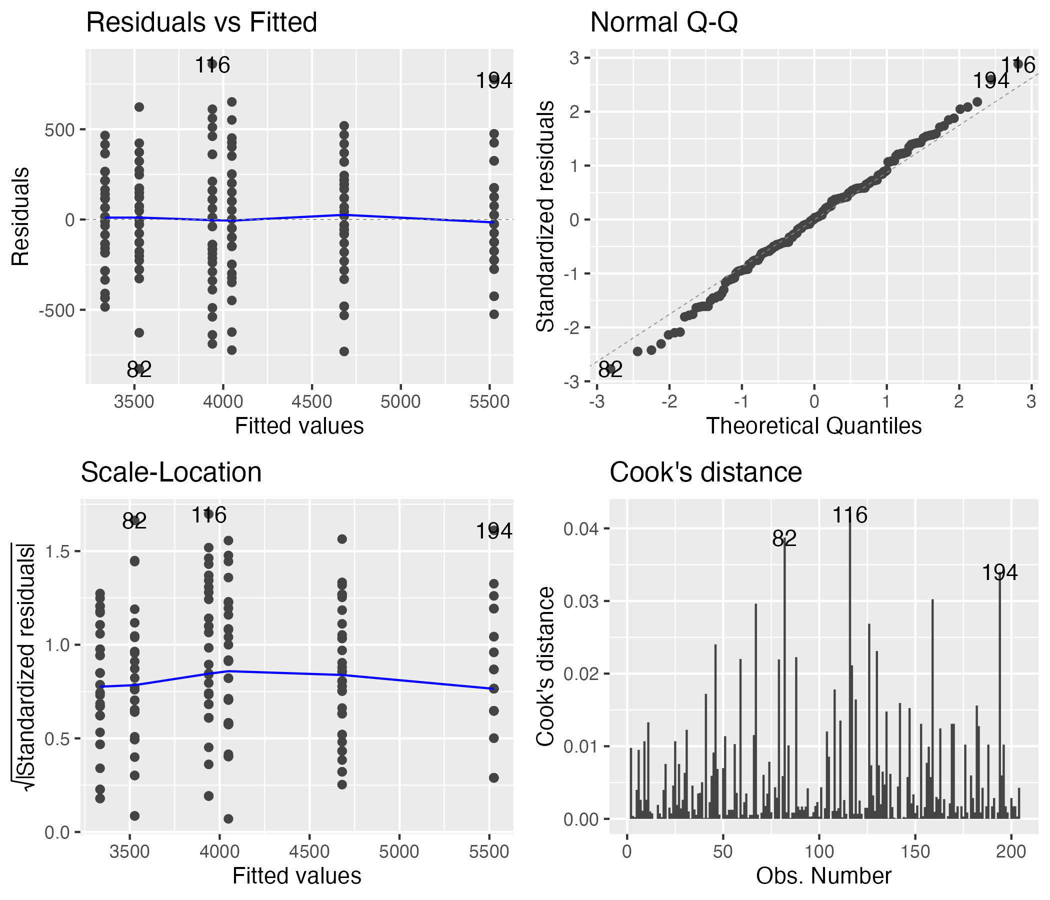
Checking Model Assumptions

The four standard diagnostic plots, built automatically with ggfortify::autoplot().

Four standard regression diagnostic plots for the two-way ANOVA model, arranged 2x2: residuals vs. fitted, normal Q-Q, scale-location, and residuals vs. leverage, generated automatically with ggfortify::autoplot().

Formal Tests — Normality and Homogeneity

The formal tests of normality of residuals and homogeneity of variances.

## Shapiro-Wilk Normality Test:
## 
##  Shapiro-Wilk normality test
## 
## data:  residuals(anova_model)
## W = 0.99612, p-value = 0.8886
## Levene's Test for Homogeneity:
## Levene's Test for Homogeneity of Variance (center = median)
##        Df F value Pr(>F)
## group   5  0.7841 0.5622
##       198
## Number of outliers (|z| > 3): 0

Part 7 · EMMs and Post-Hoc for the Balanced Model

Computing EMMs

## Species EMMs:
##  species   emmean   SE  df lower.CL upper.CL
##  Adelie      3692 36.8 198     3619     3764
##  Chinstrap   3733 36.8 198     3661     3806
##  Gentoo      5103 36.8 198     5030     5175
## 
## Results are averaged over the levels of: sex 
## Confidence level used: 0.95
## Sex EMMs:
##  sex    emmean SE  df lower.CL upper.CL
##  female   3848 30 198     3788     3907
##  male     4504 30 198     4445     4563
## 
## Results are averaged over the levels of: species 
## Confidence level used: 0.95
## Species by Sex EMMs:
##  species   sex    emmean SE  df lower.CL upper.CL
##  Adelie    female   3335 52 198     3232     3437
##  Chinstrap female   3527 52 198     3425     3630
##  Gentoo    female   4681 52 198     4578     4783
##  Adelie    male     4049 52 198     3946     4151
##  Chinstrap male     3939 52 198     3836     4042
##  Gentoo    male     5525 52 198     5422     5628
## 
## Confidence level used: 0.95

## [1] "Species pairwise comparisons:"
##  contrast           estimate SE  df t.ratio p.value
##  Adelie - Chinstrap    -41.5 52 198  -0.799  0.7041
##  Adelie - Gentoo     -1411.4 52 198 -27.145 <0.0001
##  Chinstrap - Gentoo  -1369.9 52 198 -26.346 <0.0001
## 
## Results are averaged over the levels of: sex 
## P value adjustment: tukey method for comparing a family of 3 estimates
## [1] "Species comparisons within sex:"
## sex = female:
##  contrast           estimate   SE  df t.ratio p.value
##  Adelie - Chinstrap     -193 73.5 198  -2.620  0.0256
##  Adelie - Gentoo       -1346 73.5 198 -18.310 <0.0001
##  Chinstrap - Gentoo    -1154 73.5 198 -15.690 <0.0001
## 
## sex = male:
##  contrast           estimate   SE  df t.ratio p.value
##  Adelie - Chinstrap      110 73.5 198   1.490  0.2979
##  Adelie - Gentoo       -1476 73.5 198 -20.079 <0.0001
##  Chinstrap - Gentoo    -1586 73.5 198 -21.569 <0.0001
## 
## P value adjustment: tukey method for comparing a family of 3 estimates

Post F-Test of the Interaction

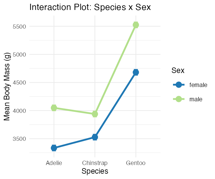
When the interaction is significant, we test the overall interaction and ignore the main effects!

##  species   sex      emmean       SE  df lower.CL upper.CL .group
##  Adelie    female 3334.559 51.99448 198 3196.378 3472.740  a    
##  Adelie    male   4048.529 51.99448 198 3910.349 4186.710   b   
##  Chinstrap female 3527.206 51.99448 198 3389.025 3665.387  a    
##  Chinstrap male   3938.971 51.99448 198 3800.790 4077.151   b   
##  Gentoo    female 4680.882 51.99448 198 4542.702 4819.063    c  
##  Gentoo    male   5525.000 51.99448 198 5386.819 5663.181     d 
## 
## Confidence level used: 0.95 
## Conf-level adjustment: sidak method for 6 estimates 
## P value adjustment: sidak method for 15 tests 
## significance level used: alpha = 0.05 
## NOTE: If two or more means share the same grouping symbol,
##       then we cannot show them to be different.
##       But we also did not show them to be the same.

The Interaction Plot

Part 8 · Unbalanced Designs

Introduction to Unbalanced Designs

The challenge of unbalanced data: real-world data is often unbalanced — unequal sample sizes across groups, missing data patterns, natural variation in sampling.

Key issues: Type I, II, and III SS give different results; order of terms matters for Type I SS; marginal means ≠ simple averages, so interpretation becomes complex.

Statistical model (same as balanced): \(Y_{ijk} = \mu + \alpha_i + \beta_j + (\alpha\beta)_{ij} + \varepsilon_{ijk}\) — but parameter estimation differs!

## [1] "Unbalanced sample sizes:"
## # A tibble: 6 × 3
##   species   sex        n
##   <fct>     <fct>  <int>
## 1 Adelie    female    73
## 2 Adelie    male      73
## 3 Chinstrap female    34
## 4 Chinstrap male      34
## 5 Gentoo    female    58
## 6 Gentoo    male      61
## [1] "Total N = 333"
## [1] "Imbalance ratio = 2.15"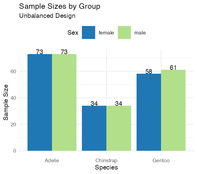

Type I (Sequential) SS

## Type I SS (Species -> Sex -> Interaction):
## Analysis of Variance Table
## 
## Response: body_mass_g
##              Df    Sum Sq  Mean Sq F value    Pr(>F)    
## species       2 145190219 72595110 758.358 < 2.2e-16 ***
## sex           1  37090262 37090262 387.460 < 2.2e-16 ***
## species:sex   2   1676557   838278   8.757 0.0001973 ***
## Residuals   327  31302628    95727                      
## ---
## Signif. codes:  0 '***' 0.001 '**' 0.01 '*' 0.05 '.' 0.1 ' ' 1
## 
## 
## Type I SS (Sex -> Species -> Interaction):
## Analysis of Variance Table
## 
## Response: body_mass_g
##              Df    Sum Sq  Mean Sq F value    Pr(>F)    
## sex           1  38878897 38878897 406.145 < 2.2e-16 ***
## species       2 143401584 71700792 749.016 < 2.2e-16 ***
## sex:species   2   1676557   838278   8.757 0.0001973 ***
## Residuals   327  31302628    95727                      
## ---
## Signif. codes:  0 '***' 0.001 '**' 0.01 '*' 0.05 '.' 0.1 ' ' 1
## 
## 
## Type I SS depends on order:
##    Effect Order1_SS Order2_SS
## 1 Species 145190219 143401584
## 2     Sex  37090262  38878897

How Type I SS works — sequential decomposition:

1. First term gets all SS it can explain
2. Second term gets SS after removing the first
3. Third term gets SS after removing the first two

Problems with unbalanced data: order dependency, biased if factors are correlated, not invariant to coding.

Type III Sums of Squares

## [1] "Type III Sums of Squares:"
## Anova Table (Type III tests)
## 
## Response: body_mass_g
##                 Sum Sq  Df   F value    Pr(>F)    
## (Intercept) 5232595969   1 54661.828 < 2.2e-16 ***
## species      143001222   2   746.924 < 2.2e-16 ***
## sex           29851220   1   311.838 < 2.2e-16 ***
## species:sex    1676557   2     8.757 0.0001973 ***
## Residuals     31302628 327                        
## ---
## Signif. codes:  0 '***' 0.001 '**' 0.01 '*' 0.05 '.' 0.1 ' ' 1
## [1] "Comparison of F-values:"
##        Effect Type_I_F Type_III_F
## 1     Species   758.36     746.92
## 2         Sex   387.46     311.84
## 3 Interaction     8.76       8.76

How Type III SS works — marginal decomposition: each effect tested after adjusting for all others.

Advantages: order invariant, tests hypotheses about unweighted means, standard in most software.

Disadvantages: lower power with missing cells, tests may not be orthogonal, requires careful interpretation.

## [1] "Effect Sizes (Type III):"
##        Effect Eta_Squared
## 1     Species      0.6947
## 2         Sex      0.1450
## 3 Interaction      0.0081

Manual SS Calculation, Step by Step

## [1] "Grand mean: 4207.1"
## [1] "Total SS: 215259666"
## [1] "Between-groups SS: 183957038"
## [1] "Within-groups SS: 31302628"
## [1] "Check: Between + Within = 215259666"

## SS(Species alone): 145190219
## SS(Sex alone): 38878897
## 
## 
## Sum of main effects: 184069116
## Actual between SS: 183957038
## 
## 
## Difference (due to correlation): -112078

Note

✅ Key idea

Main effects don’t add up to the between-groups SS here because the effects aren’t orthogonal in an unbalanced design — proof that “unbalanced” really does change the arithmetic, not just the p-values.

Part 9 · EMMs and Diagnostics — the Unbalanced Model

Estimated Marginal Means — Unbalanced Data

## Species EMMs (model-based):
##  species   emmean   SE  df lower.CL upper.CL
##  Adelie      3706 25.6 327     3656     3757
##  Chinstrap   3733 37.5 327     3659     3807
##  Gentoo      5082 28.4 327     5026     5138
## 
## Results are averaged over the levels of: sex 
## Confidence level used: 0.95
## 
## 
## Sex EMMs (model-based):
##  sex    emmean   SE  df lower.CL upper.CL
##  female   3859 25.3 327     3809     3908
##  male     4489 25.2 327     4440     4539
## 
## Results are averaged over the levels of: species 
## Confidence level used: 0.95
##  contrast                          estimate   SE  df t.ratio p.value
##  Adelie female - Chinstrap female      -193 73.5 198  -2.620  0.0973
##  Adelie female - Gentoo female        -1346 73.5 198 -18.310 <0.0001
##  Adelie female - Adelie male           -714 73.5 198  -9.710 <0.0001
##  Adelie female - Chinstrap male        -604 73.5 198  -8.220 <0.0001
##  Adelie female - Gentoo male          -2190 73.5 198 -29.789 <0.0001
##  Chinstrap female - Gentoo female     -1154 73.5 198 -15.690 <0.0001
##  Chinstrap female - Adelie male        -521 73.5 198  -7.090 <0.0001
##  Chinstrap female - Chinstrap male     -412 73.5 198  -5.600 <0.0001
##  Chinstrap female - Gentoo male       -1998 73.5 198 -27.169 <0.0001
##  Gentoo female - Adelie male            632 73.5 198   8.600 <0.0001
##  Gentoo female - Chinstrap male         742 73.5 198  10.090 <0.0001
##  Gentoo female - Gentoo male           -844 73.5 198 -11.480 <0.0001
##  Adelie male - Chinstrap male           110 73.5 198   1.490  0.6711
##  Adelie male - Gentoo male            -1476 73.5 198 -20.079 <0.0001
##  Chinstrap male - Gentoo male         -1586 73.5 198 -21.569 <0.0001
## 
## P value adjustment: tukey method for comparing a family of 6 estimates

##  species   sex      emmean       SE  df lower.CL upper.CL .group
##  Adelie    female 3368.836 36.21222 327 3272.980 3464.692  a    
##  Adelie    male   4043.493 36.21222 327 3947.637 4139.349   b   
##  Chinstrap female 3527.206 53.06120 327 3386.749 3667.662  a    
##  Chinstrap male   3938.971 53.06120 327 3798.514 4079.427   b   
##  Gentoo    female 4679.741 40.62586 327 4572.202 4787.281    c  
##  Gentoo    male   5484.836 39.61427 327 5379.975 5589.698     d 
## 
## Confidence level used: 0.95 
## Conf-level adjustment: sidak method for 6 estimates 
## P value adjustment: sidak method for 15 tests 
## significance level used: alpha = 0.05 
## NOTE: If two or more means share the same grouping symbol,
##       then we cannot show them to be different.
##       But we also did not show them to be the same.

Pairwise Comparisons — Unbalanced Data

## Species pairwise comparisons (Tukey):
##  contrast           estimate   SE  df t.ratio p.value
##  Adelie - Chinstrap    -26.9 45.4 327  -0.593  0.8241
##  Adelie - Gentoo     -1376.1 38.2 327 -36.007 <0.0001
##  Chinstrap - Gentoo  -1349.2 47.0 327 -28.682 <0.0001
## 
## Results are averaged over the levels of: sex 
## P value adjustment: tukey method for comparing a family of 3 estimates
## 
## 
## Sex effect within each species:
## species = Adelie:
##  contrast      estimate   SE  df t.ratio p.value
##  female - male     -675 51.2 327 -13.174 <0.0001
## 
## species = Chinstrap:
##  contrast      estimate   SE  df t.ratio p.value
##  female - male     -412 75.0 327  -5.487 <0.0001
## 
## species = Gentoo:
##  contrast      estimate   SE  df t.ratio p.value
##  female - male     -805 56.7 327 -14.188 <0.0001

## Sex effect (Male - Female) by species:
##     Species Sex_Effect
## 1    Adelie       -675
## 2 Chinstrap       -412
## 3    Gentoo       -805
## 
## 
## Interaction interpretation:
## [1] "Sex effects differ across species"

Diagnostic Plots — Unbalanced Design

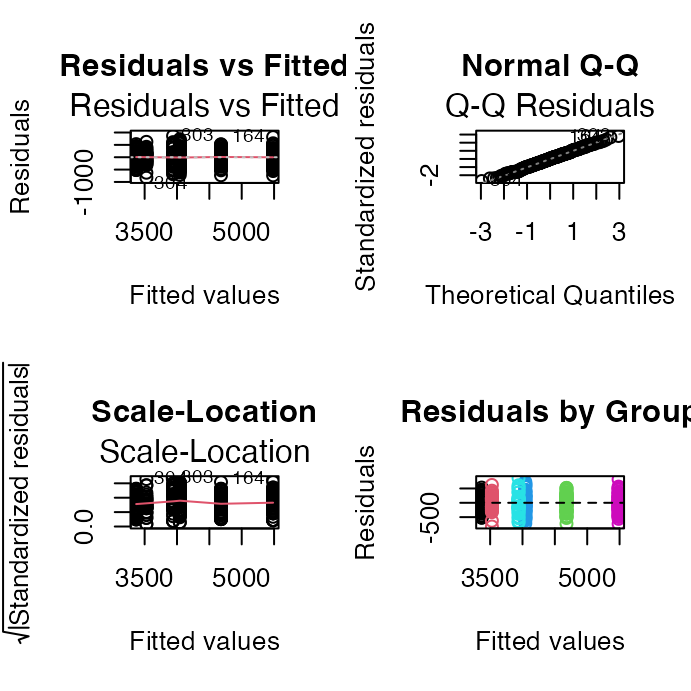
## [1] "Shapiro-Wilk test:"
## 
##  Shapiro-Wilk normality test
## 
## data:  residuals(model_u)
## W = 0.99776, p-value = 0.9367
## [1] "Levene's test:"
## Levene's Test for Homogeneity of Variance (center = median)
##        Df F value Pr(>F)
## group   5  1.3908 0.2272
##       327
## [1] "Residual SD by group:"
## # A tibble: 6 × 3
##   species   sex    sd_resid
##   <fct>     <fct>     <dbl>
## 1 Adelie    female     269.
## 2 Adelie    male       347.
## 3 Chinstrap female     285.
## 4 Chinstrap male       362.
## 5 Gentoo    female     282.
## 6 Gentoo    male       313.

Part 10 · Comparing Balanced vs. Unbalanced

Side-by-Side Comparison

## Balanced vs Unbalanced Results:
##        Effect Balanced_F Balanced_p Unbalanced_F Unbalanced_p
## 1     Species     477.20      0e+00       746.92        0e+00
## 2         Sex     239.22      0e+00       311.84        0e+00
## 3 Interaction       9.10      2e-04         8.76        2e-04
## 
## 
## Sample sizes:
## Balanced total N: 204
## Unbalanced total N: 333
## Data discarded: 129 observations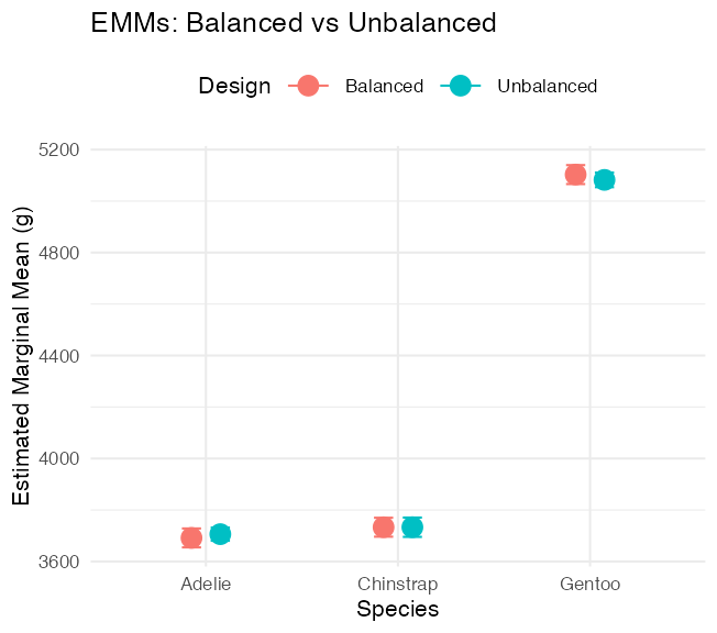

Part 11 · Summary and Best Practices

Summary — Unbalanced Designs

Challenges: Type I SS depends on order; simple means ≠ EMMs; reduced power for interactions; complex interpretation.

Solutions: use Type III SS for main effects; report EMMs, not simple means; check assumptions carefully; consider the impact of imbalance.

Recommendations:

1. Always report: sample sizes per cell, type of SS used, EMMs with CIs
2. Visualization: show actual data points, include error bars, note unequal sample sizes
3. Interpretation: focus on effect sizes, consider practical significance, acknowledge limitations

Final Recommendations

For experimental studies: design for balance when possible, randomize allocation, plan for attrition.

For observational studies: accept imbalance as reality, use Type III SS, report EMMs, consider covariates (ANCOVA).

Note

Statistical software defaults

• R: Type I (sequential)
• SAS: Type III (marginal)
• SPSS: Type III (marginal)

Always specify which type you’re using!