Lecture — One-Factor ANOVA II: Wētā, and Correcting for Size

The same eight steps, and the moment they give you the wrong answer

A second pass at one-factor ANOVA on New Zealand tree wētā, whose adult males come in three discrete morphs. We re-run last class’s eight-step recipe on foreleg length, meet two traps the possums never showed us — a circular response variable and a grouping variable confounded with body size — and then watch a hugely significant result on ear size collapse to nothing once ear is measured relative to body size. Finishes by bringing the females back as a fourth group, and on how to report a non-significant ANOVA honestly.

Where We Left Off — Possums

Eight steps, and you now know all of them:

1. factor() the groups
2. Plot it, and predict the answer
3. lm()
4. Anova(type = 2)
5. check_model() + leveneTest() + shapiro.test()
6. eta_squared()
7. emmeans() → pairs() → cld()
8. Write the sentence

Note

✅ Transition

Today we run that exact recipe on a different animal — and it hands us an answer that is statistically perfect and biologically wrong. 🦗

Goals for Today

• Run the eight steps on three wētā morphs
• Spot a response variable that is circular — the answer baked into the labels
• Spot a grouping variable confounded with body size
• Fix it with one mutate(), and watch a result vanish
• Report a non-significant ANOVA properly
• Bring the females back as a fourth group

Tools today:

• Nothing new 🎉
• Same five packages as last class

Data: 🦗 313 wētā, Te Pākeka / Maud Island, New Zealand

Tip

Four chunks: recap → the ears → the correction → the females.

Meet the Wētā 🦗

Wellington tree wētā, Hemideina crassidens — a large, flightless, nocturnal relative of crickets, found only in New Zealand.

• Lives in galleries chewed into dead wood
• A male defends a gallery holding several females
• Big enough to sit in your palm, and it will bite

313 adults were collected at night on Te Pākeka / Maud Island in March and April 2016, and 11 body parts were measured on each one.

Note

📖 Why wētā

New Zealand has almost no native land mammals. Insects took the roles mammals take elsewhere — and got big doing it.

Wētā are what happens to a cricket when nothing is hunting it from the ground.

Three Kinds of Adult Male

Wētā males stop growing at the 8th, 9th or 10th instar — three discrete adult forms, not a smooth gradient:

• eighth — small head, small jaws. Sneaks into another male’s gallery
• ninth — intermediate
• tenth — enormous head and mandibles. Fights for galleries and holds harems

Three strategies for the same job, living side by side in the same forest.

Tip

🧪 One factor, three levels

• Response: a body measurement — a number
• Factor: morph — three groups

Exactly last class’s design. The animals are stranger; the test is identical.

🧩 Chunk 1 of 4 · The Recipe Again — and Two Traps

We will cover: why we drop the females, why head_length is off-limits, and the eight steps on foreleg length.

Read It In

# Load packages ---------------------------------------
library(tidyverse)
library(car)          # Anova(), leveneTest()
library(performance)  # check_model()
library(emmeans)      # follow-up comparisons
library(multcomp)     # cld()
library(effectsize)   # eta_squared()

# Read the file ---------------------------------------
weta_raw <- read_csv("data/weta_traits.csv")

dim(weta_raw)

[1] 313  14

weta_raw %>% count(morph)

# A tibble: 4 × 2
  morph      n
  <chr>  <int>
1 eighth    78
2 female   118
3 ninth     79
4 tenth     38

Trap 1: The Females Would Swamp It

There are four groups in that file — and 118 of the 313 animals are female.

Females are much smaller than every male morph. Leave them in and the ANOVA will come back wildly significant, driven almost entirely by sex, and the three male morphs get buried.

Our question is “do the three male morphs differ?” — so the data has to be the three male morphs.

Warning

⚠️ The data must match the question

filter() is not housekeeping. It is where you decide what your test is about.

We will bring the females back in Chunk 4, on purpose, and ask a different question.

Trap 2: head_length Is Circular

The three morphs were defined using head length. From the data’s own documentation:

• eighth — male, head_length < 18.51
• ninth — male, 18.51 to 24.15
• tenth — male, head_length > 24.15

So “does head length differ among morphs?” is guaranteed. The answer was built into the labels.

You would get an enormous F and learn nothing.

Important

⚠️ Circular reasoning, in code

If the grouping variable was made from the response variable, the test is meaningless.

Nothing in R will stop you. Anova() will hand you p < 2e-16 and a gold star.

You have to catch this.

So: Males Only, Foreleg Length

weta_df <- weta_raw %>%
  filter(sex == "m", !is.na(foretibia)) %>%
  mutate(morph = factor(morph,
                        levels = c("eighth", "ninth", "tenth")))

weta_df %>% count(morph)

# A tibble: 3 × 2
  morph      n
  <fct>  <int>
1 eighth    78
2 ninth     79
3 tenth     38

Note

🧠 levels with no labels this time

The groups are already words, so factor() only needs levels — to fix the order.

Left alone R sorts alphabetically: eighth, ninth, tenth. That happens to be right. Do not rely on luck — say it out loud in the code.

Look Before You Test

ggplot(weta_df, aes(x = morph, y = foretibia)) +
  geom_boxplot(outlier.shape = NA) +
  geom_jitter(width = 0.15, alpha = 0.5)

The Group Means

weta_df %>%
  group_by(morph) %>%
  summarise(n = n(),
            mean_foretibia = round(mean(foretibia), 2),
            mean_pronotum  = round(mean(pronotum), 2))

# A tibble: 3 × 4
  morph      n mean_foretibia mean_pronotum
  <fct>  <int>          <dbl>         <dbl>
1 eighth    78           11.8          6.37
2 ninth     79           13.2          6.93
3 tenth     38           14.3          7.52

Tip

🎯 Note the second column

pronotum is the standard measure of body size in insects. It climbs too — 6.37 → 6.93 → 7.52 mm.

Hold onto that. It is the whole lesson of Chunk 3.

Fit, Test, Size

fore_model <- lm(foretibia ~ morph, data = weta_df)

Anova(fore_model, type = 2)

Anova Table (Type II tests)

Response: foretibia
           Sum Sq  Df F value    Pr(>F)    
morph     173.608   2  268.47 < 2.2e-16 ***
Residuals  62.079 192                      
---
Signif. codes:  0 '***' 0.001 '**' 0.01 '*' 0.05 '.' 0.1 ' ' 1

eta_squared(Anova(fore_model, type = 2), partial = FALSE)

# Effect Size for ANOVA (Type II)

Parameter | Eta2 |       95% CI
-------------------------------
morph     | 0.74 | [0.69, 1.00]

- One-sided CIs: upper bound fixed at [1.00].

Check the Assumptions

leveneTest(foretibia ~ morph, data = weta_df)

Levene's Test for Homogeneity of Variance (center = median)
       Df F value Pr(>F)
group   2  1.4686 0.2328
      192               

shapiro.test(residuals(fore_model))

    Shapiro-Wilk normality test

data:  residuals(fore_model)
W = 0.99345, p-value = 0.5415

Important

✅ Both pass

• Levene p = 0.233 → variances fine
• Shapiro–Wilk p = 0.542 → residuals fine

Remember the inversion: for these two, a big p is the good outcome.

Which Morphs Differ?

cld(emmeans(fore_model, ~ morph), Letters = letters)

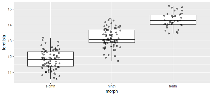
 morph  emmean     SE  df lower.CL upper.CL .group
 eighth   11.8 0.0644 192     11.7     11.9  a    
 ninth    13.2 0.0640 192     13.1     13.3   b   
 tenth    14.3 0.0922 192     14.1     14.5    c  

Confidence level used: 0.95 
P value adjustment: tukey method for comparing a family of 3 estimates 
significance level used: alpha = 0.05 
NOTE: If two or more means share the same grouping symbol,
      then we cannot show them to be different.
      But we also did not show them to be the same. 

Note

✅ a, b, c — all three separate

F(2, 192) = 268.5, p < 0.001, η² = 0.74. Morph explains 74% of the variation in foreleg length, and every morph is distinguishable from every other.

Cleanest result you will ever see. Which is exactly when you should get suspicious.

🧩 Chunk 2 of 4 · The Ears

We will cover: how a wētā hears, and a result that looks like a discovery.

Wētā Hear Through Their Knees

A wētā has no ears on its head. It hears through a tympanic membrane on the foreleg tibia — a drum on the knee.

Our file has that membrane’s area, in mm², as ear.

So we can ask a real behavioural question:

The sneaks have to listen for the fighters. Do the three morphs differ in ear size?

Tip

🧪 Why this is a good question

The three morphs play different games.

A sneak that hears a resident male coming survives. A fighter does not need to sneak.

If hearing mattered differently to them, you might see it in the hardware.

Same Recipe, New Response

ear_model <- lm(ear ~ morph, data = weta_df)

Anova(ear_model, type = 2)

Anova Table (Type II tests)

Response: ear
          Sum Sq  Df F value    Pr(>F)    
morph     23.143   2  122.19 < 2.2e-16 ***
Residuals 18.183 192                      
---
Signif. codes:  0 '***' 0.001 '**' 0.01 '*' 0.05 '.' 0.1 ' ' 1

eta_squared(Anova(ear_model, type = 2), partial = FALSE)

# Effect Size for ANOVA (Type II)

Parameter | Eta2 |       95% CI
-------------------------------
morph     | 0.56 | [0.49, 1.00]

- One-sided CIs: upper bound fixed at [1.00].

And the Letters

cld(emmeans(ear_model, ~ morph), Letters = letters)

 morph  emmean     SE  df lower.CL upper.CL .group
 eighth   2.50 0.0348 192     2.44     2.57  a    
 ninth    2.98 0.0346 192     2.92     3.05   b   
 tenth    3.42 0.0499 192     3.33     3.52    c  

Confidence level used: 0.95 
P value adjustment: tukey method for comparing a family of 3 estimates 
significance level used: alpha = 0.05 
NOTE: If two or more means share the same grouping symbol,
      then we cannot show them to be different.
      But we also did not show them to be the same. 

Important

📣 A headline result

F(2, 192) = 122.2, p < 0.001, η² = 0.56. All three morphs separate: a, b, c.

Ear area climbs 2.50 → 2.99 → 3.42 mm². Morph explains 56% of the variation.

Assumptions pass. Write the paper: “the fighting morph has a 37% larger hearing organ.”

Stop

Before you write that sentence, look back at the table from Chunk 1.

Mean pronotum — body size — by morph:

• eighth 6.37 mm
• ninth 6.93 mm
• tenth 7.52 mm

The tenth-instar males have bigger ears. They also have bigger everything. They are bigger animals.

Warning

⚠️ What did we actually test?

We asked: do the morphs differ in ear size? → Yes.

We wanted to ask: do the morphs differ in hearing?

Those are not the same question, and Anova() cannot tell them apart.

🧩 Chunk 3 of 4 · The Correction

We will cover: one mutate(), a units problem, and a result that disappears.

Measure the Ear Relative to the Animal

The fix is to divide ear size by body size — but there is a units problem first.

• ear is an area, in mm²
• pronotum is a length, in mm

Dividing an area by a length is meaningless. So first take the square root of the area, which turns it back into a length, and then divide:

ear_rel = sqrt(ear) / pronotum

Now it is a length over a length — a ratio, with no units at all.

Note

📐 Check your units

This is the oldest trick in quantitative biology and it catches errors nothing else catches.

If the units of your answer are nonsense, the answer is nonsense — however good the p-value looks.

One mutate()

weta_rel <- weta_df %>%
  mutate(ear_rel = sqrt(ear) / pronotum)

weta_rel %>%
  group_by(morph) %>%
  summarise(n = n(),
            mean_ear      = round(mean(ear), 2),
            mean_ear_rel  = round(mean(ear_rel), 4))

# A tibble: 3 × 4
  morph      n mean_ear mean_ear_rel
  <fct>  <int>    <dbl>        <dbl>
1 eighth    78     2.5         0.248
2 ninth     79     2.98        0.249
3 tenth     38     3.42        0.246

Look at Those Two Columns

Raw ear area: 2.50 → 2.99 → 3.42. Climbing hard.

Relative ear: 0.2485 → 0.2490 → 0.2459. Flat.

The third column is the same three groups, the same ear measurements, the same animals — expressed as a fraction of body size.

And there is nothing there.

Tip

🎯 Predict it now

The means are flat to three decimal places.

What is F going to be? What will the letters look like?

Run It

ear_rel_model <- lm(ear_rel ~ morph, data = weta_rel)

leveneTest(ear_rel ~ morph, data = weta_rel)

Levene's Test for Homogeneity of Variance (center = median)
       Df F value Pr(>F)
group   2  0.5249 0.5925
      192               

shapiro.test(residuals(ear_rel_model))

    Shapiro-Wilk normality test

data:  residuals(ear_rel_model)
W = 0.99313, p-value = 0.4975

The Result

Anova(ear_rel_model, type = 2)

Anova Table (Type II tests)

Response: ear_rel
             Sum Sq  Df F value Pr(>F)
morph     0.0002575   2  0.8031 0.4494
Residuals 0.0307829 192               

Important

🔄 It is gone

F(2, 192) = 0.80, p = 0.449.

Both assumptions pass — Levene p = 0.59, Shapiro p = 0.50 — so this is a trustworthy null, not a broken model.

How Big? Barely Anything

eta_squared(Anova(ear_rel_model, type = 2), partial = FALSE)

# Effect Size for ANOVA (Type II)

Parameter |     Eta2 |       95% CI
-----------------------------------
morph     | 8.30e-03 | [0.00, 1.00]

- One-sided CIs: upper bound fixed at [1.00].

Important

Morph now explains under 1% of the variation in relative ear size — down from 56% on the raw measurement.

And the Letters

cld(emmeans(ear_rel_model, ~ morph), Letters = letters)

 morph  emmean      SE  df lower.CL upper.CL .group
 tenth   0.246 0.00205 192    0.242    0.250  a    
 eighth  0.249 0.00143 192    0.246    0.251  a    
 ninth   0.249 0.00142 192    0.246    0.252  a    

Confidence level used: 0.95 
P value adjustment: tukey method for comparing a family of 3 estimates 
significance level used: alpha = 0.05 
NOTE: If two or more means share the same grouping symbol,
      then we cannot show them to be different.
      But we also did not show them to be the same. 

Note

All three share the letter a.

Same ears. Same animals. Two defensible analyses. Opposite conclusions.

p < 0.001 → p = 0.449 on one mutate().

What Changed, and What Did Not

Both results are correct. They answer different questions:

• Raw ear answers: “is a tenth-instar male’s hearing organ physically bigger?” → Yes, clearly.
• Relative ear answers: “has the hearing organ been scaled up more than the rest of the animal?” → No.

A tenth-instar male has a bigger ear for exactly the reason it has a bigger leg: it is a bigger wētā.

Warning

⚠️ Which would you report?

For a paper about hearing, the relative one — the raw result would overstate the finding badly.

For a paper about how big the organ is, the raw one.

Neither is a trick. You have to say which question you asked.

How to Report a Non-Significant ANOVA

Important

📝 Say it with the same confidence

Relative tympanic membrane size did not differ detectably among the three male morphs (one-way ANOVA, F(2, 192) = 0.80, p = 0.449, η² = 0.008), with homogeneous variances (Levene’s test p = 0.59) and normally distributed residuals (Shapiro–Wilk p = 0.50). Raw membrane area did differ (F(2, 192) = 122.2, p < 0.001), but so did body size, and the difference did not survive scaling.

Three Rules for a Null Result

• Report the numbers anyway. F, both df, p, and η². “Not significant” on its own is not a result
• Say it with the assumption checks. A null from a model that passes its checks means something. A null from a broken model means nothing
• Never write “no difference.” Write “no detectable difference”, or “we did not detect a difference”

Warning

⚠️ Absence of evidence

Remember cld()’s own note from last class:

we cannot show them to be different — but we also did not show them to be the same

With n = 38 in the smallest group, a small real difference would have slipped past us. Saying so is part of the result.

🧩 Chunk 4 of 4 · Bring the Females Back

We will cover: four groups instead of three, and a ladder that stops short.

A Different Question Needs Different Data

In Chunk 1 we dropped the females because they would swamp a question about male morphs.

Now we ask a question they belong in:

Across all four adult forms, is the foreleg scaled up differently?

The foreleg is the weapon — a tenth-instar male fights with it. If it has been built up beyond general body size, relative foreleg length should separate the groups.

Tip

🎯 Same correction, new trait

fore_rel = foretibia / pronotum

Both are lengths in mm, so no square root this time. Just divide.

Four Groups, Relative Foreleg

weta_all <- weta_raw %>%
  filter(!is.na(foretibia)) %>%
  mutate(morph = factor(morph,
                        levels = c("female", "eighth", "ninth", "tenth")),
         fore_rel = foretibia / pronotum)

weta_all %>% count(morph)

# A tibble: 4 × 2
  morph      n
  <fct>  <int>
1 female   118
2 eighth    78
3 ninth     79
4 tenth     38

fore_rel_model <- lm(fore_rel ~ morph, data = weta_all)

Check First

leveneTest(fore_rel ~ morph, data = weta_all)

Levene's Test for Homogeneity of Variance (center = median)
       Df F value  Pr(>F)  
group   3  2.2179 0.08604 .
      309                  
---
Signif. codes:  0 '***' 0.001 '**' 0.01 '*' 0.05 '.' 0.1 ' ' 1

shapiro.test(residuals(fore_rel_model))

    Shapiro-Wilk normality test

data:  residuals(fore_rel_model)
W = 0.99564, p-value = 0.5344

Note

✅ Levene p = 0.086, Shapiro p = 0.53 — both pass, so the four-group test is allowed.

Then Test

Anova(fore_rel_model, type = 2)

Anova Table (Type II tests)

Response: fore_rel
          Sum Sq  Df F value    Pr(>F)    
morph     4.0350   3  266.29 < 2.2e-16 ***
Residuals 1.5607 309                      
---
Signif. codes:  0 '***' 0.001 '**' 0.01 '*' 0.05 '.' 0.1 ' ' 1

The Ladder Stops Short

cld(emmeans(fore_rel_model, ~ morph), Letters = letters)

 morph  emmean      SE  df lower.CL upper.CL .group
 female   1.65 0.00654 309     1.64     1.67  a    
 eighth   1.86 0.00805 309     1.84     1.87   b   
 ninth    1.90 0.00800 309     1.89     1.92    c  
 tenth    1.90 0.01150 309     1.88     1.93    c  

Confidence level used: 0.95 
P value adjustment: tukey method for comparing a family of 4 estimates 
significance level used: alpha = 0.05 
NOTE: If two or more means share the same grouping symbol,
      then we cannot show them to be different.
      But we also did not show them to be the same. 

Important

a | b | c | c

F(3, 309) = 266.3, p < 0.001, η² = 0.72, both assumptions passing.

Females, then eighth, then ninth — all separate. But ninth and tenth share c: 5 of the 6 pairs are significant, and that one is not.

Relative foreleg length rises steeply, then plateaus.

What That Plateau Means

This result survived the body-size correction — unlike the ears. The foreleg really has been built up more than the animal as a whole.

But it stops. Going from ninth to tenth instar makes a wētā bigger without making its foreleg relatively longer again.

Whatever the tenth-instar morph is doing differently, by that point it is doing it with overall size, not with leg proportion.

Warning

⚠️ And the honest caveat

n = 38 for the tenth morph.

ninth and tenth sharing a letter is a failure to detect a difference. With 380 tenth-instar males it might well split.

Say that, then stop.

Your Homework

Do today over again on the hind leg — hindtibia, the jumping leg, not the weapon.

• Run the eight steps on raw hindtibia
• Then on hindtibia / pronotum
• Report both, and say what changed

Note

It will not come out like the ears.

The ears went from p < 0.001 to p = 0.449 — all the way to nothing. The hind leg does something in between. Your job is to describe it, not to match today’s answer.

Tip

🎯 One optional extra

A section on eye, where the raw analysis fails its normality check and the relative one passes.

Sometimes the right question is also the better-behaved model. Not always. But sometimes.

Recap

• The data must match the question — filter() decides what your test is about
• A circular response is meaningless — head_length defined the morphs, so never test it
• Raw size differences mostly measure body size. Divide by a body-size measure and ask again
• Check your units — ear is an area, so sqrt() before dividing by a length
• Ears: p < 0.001 → p = 0.449. Same data, one mutate(), opposite conclusion
• Forelegs: the difference survived the correction — then plateaued between ninth and tenth
• Report nulls fully — F, df, p, η², assumption checks, and “no detectable difference”

Note

✅ Next

Open the activity and run all of it. Then the hind leg. 🦗