Lecture — PCA I: Many Measurements, Few Axes

Six numbers per Pokémon, one picture, and what ‘variance explained’ means

A first, gentle pass at principal component analysis, assuming no statistics background at all. Why six correlated measurements are hard to look at, what PCA actually does (the shadow analogy), why you must scale first, running prcomp(), reading summary() for variance explained, building a scree plot, deciding how many components to keep, and checking that PC1 means something real by looking at which Pokemon sit at each end of it.

Something Completely Different

Everything this term had one response variable.

• A t-test: one measurement, two groups
• Regression: one measurement against one other
• ANOVA: one measurement across several groups

Note

✅ Transition

Today: six measurements at once, and no groups to compare. Not “is A different from B?” but “what is the shape of this whole dataset?” 🔴

Today Has No p-Values

PCA is not a test. There is nothing to reject.

• No null hypothesis
• No p-value
• No assumptions to check
• Nothing passes or fails

It is a way of looking at data that has too many columns to plot.

So the question today is never “is it significant?” It is always “does this make sense?”

Important

⚠️ Set down one habit

For nine weeks, “did it work?” meant “is p small?”

Today you judge your result by whether you can explain what the axes mean.

That is a harder standard, not an easier one.

Goals for Today

• See why six columns are hard to look at
• Notice that the columns are correlated
• Understand what PCA does — in words, not algebra
• Know why you must scale first
• Run it: prcomp()
• Read variance explained from summary()
• Draw a scree plot and decide how many axes to keep
• Sanity-check PC1 against things you already know

Tools today:

• tidyverse — that is it

Data: 🔴 the original 151 Pokémon, six battle stats each

Tip

No new packages. prcomp() is built into R.

Why Pokémon

Because you can check the answer.

PCA will hand back new axes it invented, and you have to decide whether they mean anything. That is nearly impossible to judge on unfamiliar data.

But if an axis puts Magikarp at one end and Mewtwo at the other, you know exactly what it found.

The method is the same one used on gene expression, soil chemistry, and skull measurements. Only the checking is easier.

Note

📖 The six stats

• hp — hit points
• attack — physical attack
• defense — physical defence
• sp_attack — special attack
• sp_defense — special defence
• speed — speed

Game-design numbers, but they behave exactly like six measurements off an animal.

🧩 Chunk 1 of 4 · The Problem With Six Columns

We will cover: reading the data, and why you cannot just plot it.

Read It In

library(tidyverse)

pokemon <- read_csv("data/pokemon_151.csv")

dim(pokemon)

[1] 151  15

pokemon %>%
  select(name, hp, attack, defense, sp_attack, sp_defense, speed) %>%
  head(4)

# A tibble: 4 × 7
  name          hp attack defense sp_attack sp_defense speed
  <chr>      <dbl>  <dbl>   <dbl>     <dbl>      <dbl> <dbl>
1 bulbasaur     45     49      49        65         65    45
2 ivysaur       60     62      63        80         80    60
3 venusaur      80     82      83       100        100    80
4 charmander    39     52      43        60         50    65

Six Columns Is Too Many to Plot

One measurement → a histogram.

Two → a scatterplot.

Three → an awkward 3-D scatterplot nobody can read.

Six → nothing. There is no six-dimensional plot, and there never will be.

You could draw all the pairs instead. Six columns make 15 pairwise scatterplots, and no one can hold 15 plots in their head at once.

Warning

⚠️ The real problem

It is not that drawing is hard.

It is that “which Pokémon are similar to each other?” is a question about all six numbers at the same time, and looking at them two at a time cannot answer it.

Make Them a Table of Their Own

poke_stats <- pokemon %>%
  select(hp, attack, defense, sp_attack, sp_defense, speed)

dim(poke_stats)

[1] 151   6

Note

🧠 Why a separate table

PCA needs numbers only — no names, no types. poke_stats is 151 rows and exactly 6 numeric columns.

The rows stay in the same order as pokemon, which is what lets us glue the results back on later.

Do the Stats Move Together?

poke_stats %>%
  cor() %>%
  round(2)

              hp attack defense sp_attack sp_defense speed
hp          1.00   0.30    0.12      0.24       0.49 -0.04
attack      0.30   1.00    0.48      0.14       0.37  0.20
defense     0.12   0.48    1.00      0.19       0.14 -0.05
sp_attack   0.24   0.14    0.19      1.00       0.53  0.41
sp_defense  0.49   0.37    0.14      0.53       1.00  0.39
speed      -0.04   0.20   -0.05      0.41       0.39  1.00

Reading That Matrix

The diagonal is all 1.00 — every column correlates perfectly with itself. Ignore it.

Everything else is the interesting part:

• sp_attack and sp_defense: 0.53
• hp and sp_defense: 0.49
• attack and defense: 0.48
• speed and defense: −0.05 — nothing at all

So the six columns are not six independent facts. They overlap. Knowing one tells you something about the others.

Important

✅ This is what makes PCA work

If all six columns were completely unrelated, PCA would have nothing to do — six axes in, six equally useless axes out.

Correlation is redundancy. PCA’s whole job is to squeeze the redundancy out.

🧩 Chunk 2 of 4 · What PCA Actually Does

We will cover: the shadow analogy, and why scaling comes first.

The Shadow Analogy 🔦

Hold your hand up in front of a lamp and look at the shadow on the wall.

Your hand is 3-D. The shadow is 2-D. You have lost a dimension — but you can still tell it is a hand.

Now rotate your hand. Some angles give a shadow you can recognise instantly. Others give a shapeless blob.

Same hand. Same wall. Different amount of information kept.

Tip

🎯 That is PCA

Your data is a cloud of 151 points in 6-D space.

PCA finds the angle that casts the most informative shadow — the one where the points stay as spread out as possible.

Then it reports what that shadow is made of.

Said Without the Analogy

PCA builds new measurements by blending the old ones:

\[\text{PC1} = a_1\,\text{hp} + a_2\,\text{attack} + \ldots\]

It picks the weights so that:

• PC1 captures as much of the spread between Pokémon as any single blend can
• PC2 captures as much of what is left over as possible — and is at right angles to PC1
• PC3 takes the next-biggest leftover, and so on

Six columns in, six PCs out — but they come in order of usefulness.

Note

🧠 Two words you need

Loading — how much an original stat contributes to a PC. What the axis is made of.

Score — where one Pokémon sits along that PC. Its new measurement.

Loadings describe the axis. Scores describe the Pokémon. That is all of Chunk 2 of next class.

First: You Must Scale

poke_stats %>%
  summarise(across(everything(),
                   ~ round(sd(.x), 1)))

# A tibble: 1 × 6
     hp attack defense sp_attack sp_defense speed
  <dbl>  <dbl>   <dbl>     <dbl>      <dbl> <dbl>
1  28.6   26.8    26.9      28.5       24.2    27

hp varies more than defense does — in raw points.

PCA chases spread. Hand it unscaled columns and it will decide the most important thing in the data is whichever column happens to use the biggest numbers.

Warning

⚠️ A worked disaster

Imagine measuring animals in grams and kilometres.

Body mass in grams: thousands. Home range in km: maybe 0.4.

Unscaled, PC1 would be entirely mass, and would tell you nothing except which unit you typed.

Scaling, In One Argument

scale. = TRUE converts every column to standard deviations from its own mean before doing anything else.

After scaling, every column has:

• mean 0
• standard deviation 1

Now all six compete fairly, and the units cancel out entirely.

Important

⚠️ Mind the full stop

The argument is scale. — with a dot:

prcomp(poke_stats, scale. = TRUE)

The dot is there because scale was already an R function. Leave it off and you get an error.

Almost always use scale. = TRUE.

🧩 Chunk 3 of 4 · Run It and Read It

We will cover: prcomp(), summary(), variance explained, and the scree plot.

One Line

poke_pca <- prcomp(poke_stats, center = TRUE, scale. = TRUE)

Note

🧠 That is the entire analysis

• center = TRUE — subtract each column’s mean
• scale. = TRUE — divide by each column’s standard deviation

Everything from here on is reading the result, which is the part that takes judgement.

What Came Back

summary(poke_pca)

Importance of components:
                          PC1    PC2    PC3    PC4     PC5
Standard deviation     1.5418 1.1349 0.9943 0.8280 0.58318
Proportion of Variance 0.3962 0.2147 0.1648 0.1143 0.05668
Cumulative Proportion  0.3962 0.6109 0.7756 0.8899 0.94655
                           PC6
Standard deviation     0.56630
Proportion of Variance 0.05345
Cumulative Proportion  1.00000

Reading summary() — the Only Row That Matters

Ignore the first row. Read these two:

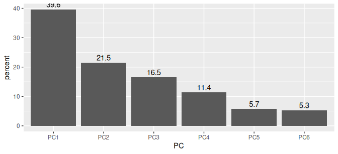
Proportion of Variance — how much of the total spread each PC captures:

• PC1: 39.6%
• PC2: 21.5%
• PC3: 16.5%

Cumulative Proportion — the running total:

• PC1 alone: 39.6%
• PC1 + PC2: 61.1%
• All six: 100%, always

Important

✅ The headline

Two invented axes carry 61% of everything in six columns.

So a flat scatterplot of PC1 against PC2 — which we draw next class — shows you about three-fifths of the whole dataset.

That is the payoff.

“Variance Explained”, In Plain Words

Variance here just means how spread out things are.

Total variance = every way these 151 Pokémon differ from each other across all six stats.

PC1 captures 39.6% of that. Meaning: if you threw away all six stats and kept only each Pokémon’s PC1 score, you would still have about 40% of the information about how they differ.

One number instead of six, for 40% of the picture.

Warning

⚠️ Not 39.6% of the Pokémon

And not 39.6% accuracy.

It is 39.6% of the total variation — of the differences between them.

If every Pokémon had identical stats there would be no variance at all, and PCA would have nothing to find.

How Much Variance Per Axis

var_df <- tibble(
  PC      = paste0("PC", 1:6),
  percent = round(100 * poke_pca$sdev^2 / sum(poke_pca$sdev^2), 1)
)

var_df

# A tibble: 6 × 2
  PC    percent
  <chr>   <dbl>
1 PC1      39.6
2 PC2      21.5
3 PC3      16.5
4 PC4      11.4
5 PC5       5.7
6 PC6       5.3

Note

🧠 Where that came from

poke_pca$sdev is each PC’s standard deviation. Squaring it gives variance; dividing by the total turns it into a share; times 100 is a percent.

It is the same numbers summary() printed — but now in a data frame, which means we can plot them.

The Scree Plot

ggplot(var_df, aes(x = PC, y = percent)) +
  geom_col() +
  geom_text(aes(label = percent), vjust = -0.4)

Reading a Scree Plot

A scree plot is variance explained, per axis, in order. (“Scree” is the loose rubble at the foot of a cliff — the shape the bars make.)

You are looking for the elbow: where the bars stop dropping steeply and flatten into rubble.

Here PC1 and PC2 stand up; from PC3 on the bars settle down and get similar. So the honest answer is keep two, and know you are holding 61%.

Warning

⚠️ There is no rule

Nothing tells you where the elbow is. People argue about it constantly.

Common rough guides:

• Keep PCs until the cumulative total passes ~70–80%
• Keep the ones before the flat part
• Keep the ones you can interpret

That last one is the most useful.

🧩 Chunk 4 of 4 · Does PC1 Mean Anything?

We will cover: the only check that matters — looking at who sits at each end.

A Quick Look at What PC1 Is Made Of

round(poke_pca$rotation[, 1:2], 2)

            PC1   PC2
hp         0.38  0.19
attack     0.42  0.43
defense    0.28  0.59
sp_attack  0.45 -0.33
sp_defense 0.54 -0.17
speed      0.32 -0.54

Important

✅ Look at the PC1 column: every single number is positive

So a Pokémon scores high on PC1 by being high on all six stats at once.

PC1 is an “overall power” axis. We will take this table apart properly next class — for now, notice that PC2 has minus signs, which means it is doing something completely different.

Where Does Each Pokémon Sit?

poke_scores <- pokemon %>%
  mutate(PC1 = poke_pca$x[, 1],
         PC2 = poke_pca$x[, 2])

poke_scores %>%
  select(name, hp, attack, speed, PC1, PC2) %>%
  head(3)

# A tibble: 3 × 6
  name         hp attack speed    PC1    PC2
  <chr>     <dbl>  <dbl> <dbl>  <dbl>  <dbl>
1 bulbasaur    45     49    45 -1.18  -0.417
2 ivysaur      60     62    60  0.123 -0.384
3 venusaur     80     82    80  1.91  -0.269

Note

🧠 poke_pca$x holds the scores

One row per Pokémon, one column per PC — in the same row order as the data we put in. That is why we could glue it straight on with mutate().

The Top of PC1

poke_scores %>%
  arrange(desc(PC1)) %>%
  select(name, is_legendary, PC1) %>%
  head(6)

# A tibble: 6 × 3
  name      is_legendary   PC1
  <chr>     <lgl>        <dbl>
1 mewtwo    TRUE          4.00
2 dragonite FALSE         3.00
3 mew       FALSE         2.88
4 articuno  TRUE          2.81
5 zapdos    TRUE          2.60
6 moltres   TRUE          2.58

The Bottom of PC1

poke_scores %>%
  arrange(PC1) %>%
  select(name, PC1) %>%
  head(6)

# A tibble: 6 × 2
  name       PC1
  <chr>    <dbl>
1 magikarp -3.43
2 caterpie -3.34
3 weedle   -3.32
4 metapod  -3.21
5 kakuna   -3.19
6 zubat    -2.45

That Is the Whole Validation 🎣

Top of PC1: Mewtwo, Dragonite, Mew, Articuno, Zapdos, Moltres — every legendary in the game, plus the two strongest non-legendaries.

Bottom of PC1: Magikarp, Caterpie, Weedle, Metapod, Kakuna, Zubat.

Nobody told PCA which Pokémon were strong. There is no “power” column in the file. It was handed six columns of numbers and it sorted them by overall strength on its own.

Important

✅ Why this matters beyond Pokémon

This is the check you run on every PCA.

You cannot test whether an axis is “real”. But you can look at what sits at each end and ask whether it lines up with something you already know.

If it does, the axis is measuring something. If it does not, be very careful.

Put a Number on It

poke_scores %>%
  group_by(is_legendary) %>%
  summarise(n = n(),
            mean_PC1 = round(mean(PC1), 2))

# A tibble: 2 × 3
  is_legendary     n mean_PC1
  <lgl>        <int>    <dbl>
1 FALSE          147    -0.08
2 TRUE             4     3   

Note

The four legendaries average PC1 = 3.00; everyone else averages −0.08.

PC1 scores are in standard deviations, so the legendaries sit about three standard deviations above the crowd — on an axis that was built without ever being told they existed.

What We Have, and What Is Missing

We have:

• Two axes holding 61% of six columns
• PC1 identified as “overall power”, checked against Magikarp and Mewtwo

We do not have:

• Any idea what PC2 means
• A picture — we have not plotted a single Pokémon yet
• Any way to see the original six stats on that picture

All three are next class.

Tip

🎯 A hint about PC2

Look back at the loadings. In PC2, defense is +0.59 and speed is −0.54.

A big positive and a big negative on the same axis means PC2 is a trade-off, not a total.

Which trade-off? Next class.

Your Homework

Do today again on all 1,025 Pokémon instead of the original 151.

data/pokemon_1025.csv has the identical columns, so the homework is mostly changing one filename and re-reading your output.

The real question: does PC1 still mean the same thing? Twenty-five years of new Pokémon, nine generations — or is “overall power” just a quirk of the first 151?

Note

📂 What you will do

The whole chunk-1-to-4 sequence on the bigger file, then compare your percentages and your top/bottom lists to today’s.

All the code is in the homework file. Most of the marks are for reading what comes out.

Recap

• PCA is not a test — no p-value, no assumptions, nothing to reject
• It exists because six columns cannot be plotted, and pairs cannot answer “who is similar to whom”
• It works because the columns are correlated — correlation is redundancy
• Think shadows: a lower-dimensional view, taken from the most informative angle
• Always scale. = TRUE, or the column with the biggest numbers wins by default
• prcomp() is one line; reading it is the work
• PC1 = 39.6%, PC2 = 21.5%, together 61.1% of everything in six columns
• The scree plot shows where to stop; there is no rule, only judgement
• Validate by looking at the ends. Magikarp at one end, Mewtwo at the other ✅

Note

✅ Next

Open the activity and run it. Next class: what PC2 means, and the picture. 🔴