Lecture — PCA II: Loadings, Scores, and the Biplot

What PC2 means, and finally drawing the picture

The second half of PCA, still assuming no statistics background. Reading a loadings table properly, recognising that a mix of positive and negative loadings means a trade-off rather than a total, naming PC2 from its loadings and then confirming it from the Pokemon at each end, plotting the scores, labelling extremes with ggrepel, building a biplot by hand so the arrows are not magic, and writing a PCA up when there is no p-value to lean on.

Where We Left Off

• Six correlated stats, impossible to plot
• PCA found new axes by blending them — the most informative shadow
• prcomp(poke_stats, center = TRUE, scale. = TRUE)
• PC1 = 39.6%, PC2 = 21.5%, together 61.1%
• PC1 had all-positive loadings → “overall power”
• Checked it: Magikarp at the bottom, Mewtwo at the top ✅

Note

✅ Transition

Three things were missing: what PC2 means, a picture, and a way to see the original stats on that picture. All three today. 🔴

Goals for Today

• Read a loadings table properly
• Learn the one rule: mixed signs mean a trade-off
• Name PC2 from its loadings, then prove it from the data
• Plot the Pokémon in PC space — the picture at last
• Label the interesting points with ggrepel
• Build a biplot by hand, so the arrows are not magic
• Write up a PCA when there is no p-value to lean on

Tools today:

• tidyverse
• ggrepel — install this

Data: 🔴 the same 151 Pokémon

Important

⚠️ Install first

install.packages("ggrepel")

Small and fast — but do it before class.

We Have to Re-run It

library(tidyverse)
library(ggrepel)

pokemon <- read_csv("data/pokemon_151.csv")

poke_stats <- pokemon %>%
  select(hp, attack, defense, sp_attack, sp_defense, speed)

poke_pca <- prcomp(poke_stats, center = TRUE, scale. = TRUE)

Note

🧠 Every script starts from the raw data

Nothing today depends on objects left over in last class’s session. Restart R, run from the top, and you get the same answer.

If a script only works because of something you ran yesterday, it is broken — you just cannot see it yet.

🧩 Chunk 1 of 4 · Reading the Loadings

We will cover: the loadings table in full, the mixed-sign rule, and naming PC2.

The Loadings Table

round(poke_pca$rotation[, 1:3], 2)

            PC1   PC2   PC3
hp         0.38  0.19  0.72
attack     0.42  0.43 -0.26
defense    0.28  0.59 -0.41
sp_attack  0.45 -0.33 -0.06
sp_defense 0.54 -0.17  0.23
speed      0.32 -0.54 -0.44

Note

One row per original stat. One column per PC.

A loading is how much that stat contributes to that axis. Big number = matters a lot. Near zero = barely involved. The sign tells you which direction.

PC1: All the Same Sign

Read down the PC1 column:

Stat	Loading
sp_defense	0.54
sp_attack	0.45
attack	0.42
hp	0.38
speed	0.32
defense	0.28

Every one positive, and none of them tiny. To score high on PC1 you must be high on everything.

Important

✅ The rule for all-positive

An axis where every loading shares a sign is a “total” axis — an overall size, overall strength, overall abundance.

You will see this constantly. PC1 is very often a total, because the single biggest way things differ is usually just how much of them there is.

PC2: Mixed Signs

Now read down PC2:

Stat	Loading
defense	+0.59	⬆️
attack	+0.43	⬆️
hp	+0.19
sp_defense	−0.17
sp_attack	−0.33	⬇️
speed	−0.54	⬇️

Two big positives and two big negatives on the same axis.

Important

✅ The rule for mixed signs

Mixed signs mean a trade-off, not a total.

PC2 is not measuring how much. It is measuring which kind — being strong in one way instead of another.

High PC2 = defense + attack. Low PC2 = speed + sp_attack.

Naming PC2

So high PC2 means tough and hard-hitting but slow. Low PC2 means fast and special-attacking but fragile.

Anyone who has played the game has a name for these:

• High PC2 → a tank
• Low PC2 → a glass cannon

PC2 is a “tank ↔︎ glass cannon” axis, and it carries 21.5% of all the variation in six columns.

Warning

⚠️ You named it. The maths did not.

prcomp() returned a column of numbers labelled PC2. It has no idea what a tank is.

Naming an axis is interpretation, and it is your responsibility. It is also the single most valuable thing you do in a PCA — and the easiest place to fool yourself.

Prove It From the Data

poke_scores <- pokemon %>%
  mutate(PC1 = poke_pca$x[, 1],
         PC2 = poke_pca$x[, 2])

poke_scores %>%
  arrange(desc(PC2)) %>%
  select(name, defense, speed, PC2) %>%
  head(4)

# A tibble: 4 × 4
  name     defense speed   PC2
  <chr>      <dbl> <dbl> <dbl>
1 rhydon       120    40  3.31
2 golem        130    45  2.84
3 cloyster     180    70  2.63
4 rhyhorn       95    25  2.46

And the Other End

poke_scores %>%
  arrange(PC2) %>%
  select(name, defense, speed, PC2) %>%
  head(4)

# A tibble: 4 × 4
  name     defense speed   PC2
  <chr>      <dbl> <dbl> <dbl>
1 abra          15    90 -3.05
2 kadabra       30   105 -2.97
3 alakazam      45   120 -2.95
4 jynx          35    95 -2.37

That Is a Confirmed Axis 🪨⚡

Top of PC2: Rhydon, Golem, Cloyster, Rhyhorn — defence 95 to 180, speed 25 to 70. Rocks.

Bottom of PC2: Abra, Kadabra, Alakazam, Jynx — defence 15 to 45, speed 90 to 120.

Alakazam is the fastest, most fragile special attacker in the game. Golem is a literal boulder. They are at opposite ends of an axis that was built from nothing but six columns of numbers.

Important

✅ The two-step, every time

1. Read the loadings → form a guess about what the axis means
2. Look at the extremes → check the guess against things you know

Do them in that order. If step 2 disagrees with step 1, believe step 2.

🧩 Chunk 2 of 4 · Finally, the Picture

We will cover: plotting 151 Pokémon on two invented axes.

The Plot We Have Been Working Towards

ggplot(poke_scores, aes(x = PC1, y = PC2)) +
  geom_point(alpha = 0.7)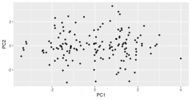

What You Are Looking At

Every dot is one Pokémon. Neither axis is a thing anyone measured — both were invented by prcomp().

• Left ↔︎ right = weak ↔︎ strong (PC1, 39.6%)
• Bottom ↔︎ top = glass cannon ↔︎ tank (PC2, 21.5%)

Two dots close together = two Pokémon with similar stat profiles overall. That is the question we could not answer with 15 pairwise scatterplots.

And this flat picture holds 61% of six columns.

Note

🧠 The origin is average

The scores were centred, so (0, 0) is the average Pokémon — not zero power.

A dot at the far left is not “no stats”. It is well below average.

Colour by Something You Know

ggplot(poke_scores, aes(x = PC1, y = PC2, color = is_legendary)) +
  geom_point(alpha = 0.7, size = 2)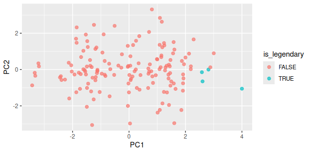

Four Dots on the Right

The four legendaries sit in a cluster at the far right — high PC1 — and slightly low on PC2.

So the game’s strongest Pokémon are not just powerful; they lean a little towards the fast, special-attacking side rather than the tank side.

Nothing in the PCA knew which Pokémon were legendary. The is_legendary column was never given to prcomp() — we only used it to colour the result.

Important

✅ That is the right way round

Build the axes from the measurements only. Then colour by the thing you care about and see whether it lines up.

Put the grouping variable into the PCA and you have built the answer you wanted — the same circular trap as the wētā’s head_length.

🧩 Chunk 3 of 4 · Label the Interesting Ones

We will cover: why 151 labels is unreadable, and ggrepel.

Do Not Label Everything

The obvious next step is to put names on the dots. With 151 Pokémon, that gives you a solid black rectangle.

So label only the extremes — the ones furthest from the centre, which are the ones a reader will ask about.

One way to pick them: keep anything in the top 3% on either axis, in either direction.

Note

🧠 abs() and quantile()

abs(PC1) is distance from the centre, ignoring direction.

quantile(abs(PC1), 0.97) is the value only 3% of Pokémon exceed.

Together: “far from average on PC1, either way.”

Pick the Extremes

extremes <- poke_scores %>%
  filter(abs(PC1) > quantile(abs(PC1), 0.97) |
         abs(PC2) > quantile(abs(PC2), 0.97))

nrow(extremes)

[1] 10

extremes %>%
  select(name, PC1, PC2) %>%
  head(5)

# A tibble: 5 × 3
  name         PC1    PC2
  <chr>      <dbl>  <dbl>
1 caterpie -3.34   -0.180
2 metapod  -3.21    0.339
3 weedle   -3.32   -0.344
4 abra     -1.31   -3.05 
5 kadabra   0.0355 -2.97 

Now Label Just Those

ggplot(poke_scores, aes(x = PC1, y = PC2)) +
  geom_point(color = "grey70") +
  geom_point(data = extremes, color = "firebrick") +
  geom_text_repel(data = extremes, aes(label = name), size = 3)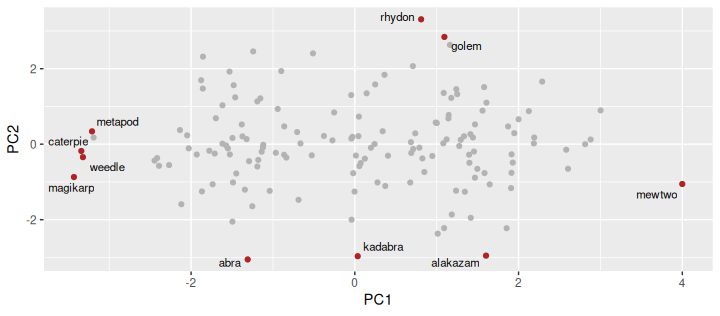

How That Plot Is Built

Three layers, and the order matters:

• geom_point(color = "grey70") — all 151, in the background
• geom_point(data = extremes, ...) — the interesting ones, on top, in red
• geom_text_repel(data = extremes, ...) — names, only for those

geom_text_repel() is ggrepel’s version of geom_text(). It nudges labels apart so they do not sit on top of each other, and draws a little line back to the dot.

Tip

🎯 data = inside a layer

Each geom_ can take its own data =. Give it one and that layer ignores the data in ggplot().

That is how you draw two different subsets on one plot — and it works for every geom, not just these.

🧩 Chunk 4 of 4 · The Biplot

We will cover: putting the original six stats back onto the picture.

The Problem a Biplot Solves

Our plot shows where Pokémon sit. It does not show which direction each original stat points.

A biplot draws both at once:

• Points = the Pokémon (the scores)
• Arrows = the original stats (the loadings)

An arrow points the way that stat increases. Long arrow = strongly involved in these two axes. Arrows pointing the same way = correlated stats.

Note

🧠 “Bi”-plot

Two things on one plot, in two different units.

R has a built-in biplot(poke_pca). It is ugly and hard to control, so we will build ours from the loadings — which also means you will know exactly what the arrows are.

Turn the Loadings Into Arrows

arrows_df <- as_tibble(poke_pca$rotation[, 1:2], rownames = "stat") %>%
  mutate(PC1 = PC1 * 4,
         PC2 = PC2 * 4)

arrows_df

# A tibble: 6 × 3
  stat         PC1    PC2
  <chr>      <dbl>  <dbl>
1 hp          1.51  0.770
2 attack      1.68  1.70 
3 defense     1.14  2.36 
4 sp_attack   1.80 -1.33 
5 sp_defense  2.16 -0.690
6 speed       1.30 -2.16 

Warning

⚠️ Why * 4

Loadings run about −0.6 to +0.6. The scores run about −3.5 to +3.5. Draw the arrows at their true length and they vanish into a dot at the centre.

Multiplying by 4 is purely cosmetic — it makes them visible. It changes the arrows’ lengths on screen, never their directions, and the directions are the part you interpret.

The Biplot

ggplot(poke_scores, aes(x = PC1, y = PC2)) +
  geom_point(color = "grey75", alpha = 0.7) +
  geom_segment(data = arrows_df,
               aes(x = 0, y = 0, xend = PC1, yend = PC2),
               arrow = arrow(length = unit(0.2, "cm"))) +
  geom_text_repel(data = arrows_df, aes(label = stat),
                  fontface = "bold", size = 3.4)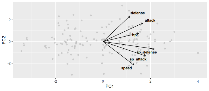

Reading the Arrows

• Every arrow points right. All six stats increase with PC1 — the all-positive loadings, now visible
• defense points up-right, speed points down-right. They are nearly opposite vertically — the trade-off
• attack sits with defense; sp_attack and sp_defense lean with speed
• defense has the longest arrow, hp the shortest — so hp is the stat least involved in these two axes

Important

✅ Angles, not positions

• Arrows close together → correlated stats
• Arrows at right angles → unrelated
• Arrows opposite → trade-off

Check it against Part 4 of last class: speed and defense had r = −0.05… yet here they look opposed. Why? Because the biplot shows only these two axes — 61% of the picture, not all of it.

A Trap Worth Naming

speed and defense have a real correlation of −0.05 — essentially unrelated.

But on this biplot their arrows point in nearly opposite directions, which looks like a strong trade-off.

Both are true. The biplot is a shadow. Two arrows can look opposed in the shadow while being unrelated in the full six dimensions.

Warning

⚠️ So always say how much you are showing

“PC1 and PC2, which together explain 61.1% of the variance”

Without that number, a reader cannot tell whether your biplot is the whole story or three-fifths of it.

Never show a biplot without its percentages.

Writing Up a PCA

Important

📝 No p-value, so the structure is different

Six battle statistics for the 151 original Pokémon were standardised and reduced by principal component analysis. The first two components explained 61.1% of the total variance (PC1 39.6%, PC2 21.5%). PC1 loaded positively on all six statistics (0.28 to 0.54) and is interpreted as overall power: the four legendary Pokémon averaged PC1 = 3.00 against −0.08 for all others, and Magikarp held the lowest score. PC2 contrasted defense (+0.59) and attack (+0.43) against speed (−0.54) and sp_attack (−0.33), separating durable, slow-moving species such as Golem and Cloyster from fast, fragile ones such as Alakazam.

What That Paragraph Does

• Says what went in — six stats, 151 Pokémon
• Says it was standardised (scale. = TRUE)
• Gives variance explained, per axis and cumulative
• Names each axis, and gives the loadings that justify the name
• Gives evidence from the data — real Pokémon at each end
• Never says “significant”, because nothing was tested

Warning

⚠️ The two failure modes

Too little: “We ran a PCA and PC1 explained 39.6%.” Explained of what? Meaning what?

Too much: “PC1 proves power is one-dimensional.” PCA proves nothing. It describes.

Describe, name, justify. Stop there.

Your Homework

Take all 1,025 Pokémon — the file from last class’s homework — and do today’s four chunks on it:

• Read the loadings and name PC2 for yourself
• Confirm it from the extremes
• Draw the scores plot, coloured by legendary — this time 71 of them, not 4
• Draw the biplot

All the code is written. The marks are for the naming and the write-up.

Tip

🎯 One thing to watch for

With 1,025 Pokémon your scores plot has 1,025 dots. It will look crowded.

One of the questions asks what you would change to make it readable — and “label fewer things” is a perfectly good answer.

Recap

• A loading is what an axis is made of; a score is where one row sits on it
• All loadings the same sign → a “total” axis. PC1 usually is
• Mixed signs → a trade-off. PC2 here is tank ↔︎ glass cannon
• Name the axis from the loadings, then confirm from the extremes — and if they disagree, believe the extremes
• Build the axes from measurements only; colour by your grouping variable afterwards
• Label only the extremes — geom_text_repel(), with its own data =
• A biplot = points (scores) + arrows (loadings). Read angles, not positions
• Arrows can look opposed in a 2-D shadow while being unrelated in 6-D — always report the percentages
• Write-ups describe and justify. Nothing was tested, so nothing is significant ✅

Note

✅ Next

Open the activity and run it. Then all 1,025. 🔴