Lecture: Linear Mixed Models

Random effects for nested and hierarchical data

The modern mixed-model (lmer) alternative to a traditional nested ANOVA: afex for unbalanced designs, random-effects notation, F vs. Chi-square tests, diagnostics, post-hoc comparisons, and a by-hand F-ratio calculation for comparison — on the sea urchin grazing / algae cover dataset.

Where We Left Off

Covered last time — nested ANOVA, the traditional way:

• Factorial vs. nested designs
• The nested-design linear model and variance partitioning
• Fixed vs. random effects — B nested in A
• The naive (wrong) factorial model vs. aov(..., Error(...))

Note

✅ Key idea from last lecture

patch nested in treat needs the right error term — MS_{patch(treat)}, not MS_{resid} — or the F-test for treatment is wrong. Today: the modern alternative to specifying that error term by hand.

Tip

🖐 Notice

Same sea urchin grazing / algae cover dataset as last time — same question, same data, a different (and more flexible) way to fit the model.

Part 1 · Setup — The Sea Urchin Data, Again

Data Overview

Same dataset as the nested ANOVA lecture: patch (random patches 1–16 where treatments were applied), treat (urchin density treatment), quad (replicate quadrats within each treatment-patch combination), algae (percentage cover of filamentous algae — the response variable).

## Data
## # A tibble: 6 × 4
##   treat patch  quad algae
##   <fct> <fct> <dbl> <dbl>
## 1 100%  1         1     0
## 2 100%  1         2     0
## 3 100%  1         3     0
## 4 100%  1         4     6
## 5 100%  1         5     2
## 6 100%  2         1     0
## 
## 
## Treatment levels:
## [1] "0%"   "33%"  "66%"  "100%"

## Summary statistics by treatment:
## # A tibble: 4 × 7
##   treat     n  mean    sd    se   min   max
##   <fct> <int> <dbl> <dbl> <dbl> <dbl> <dbl>
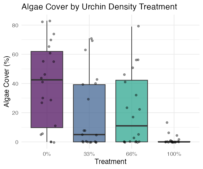
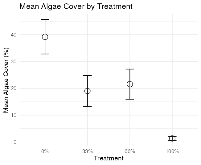
## 1 0%       20  39.2 28.7  6.41      0    83
## 2 33%      20  19   25.7  5.74      0    71
## 3 66%      20  21.6 25.1  5.62      0    79
## 4 100%     20   1.3  3.18 0.711     0    13

Part 2 · Modern Approaches — afex and Mixed Models

What to Do If It’s an Unbalanced Design

The afex package is specifically designed for ANOVA with Type III SS, and handles nested designs well — even when unbalanced.

options(contrasts = c("contr.sum", "contr.poly"))

u_afex_model <- aov_car(algae ~ treat + Error(patch),
                     data = u_df,
                     fun_aggregate = mean)
cat("AFEX nested ANOVA results:\n\n")
## AFEX nested ANOVA results:
summary(u_afex_model)
## Anova Table (Type 3 tests)
## 
## Response: algae
##       num Df den Df    MSE      F     ges  Pr(>F)  
## treat      3     12 354.03 2.7171 0.40451 0.09126 .
## ---
## Signif. codes:  0 '***' 0.001 '**' 0.01 '*' 0.05 '.' 0.1 ' ' 1

What Makes an Effect “Random”?

Ask one question: do I care about these specific levels, or are they a sample of levels I could have had?

	treat	patch
The levels are	0/33/66/100% density	patches 1–16
Chosen by	me, deliberately	whatever was there
Would a repeat study use the same ones?	yes	no — different patches
I want to estimate	each level’s mean	how much they vary
So it is	fixed	random

Important

The key consequence

A fixed factor with 16 levels costs you 15 parameters. A random factor with 16 levels costs you one — a single variance, σ²_patch.

That is why mixed models cope with designs that aov() chokes on: they are estimating far less.

Note

📖 A useful test

If you can write a sentence a reader would care about that names a specific level — “the 100% density treatment reduced algae” — it is fixed.

If the sentence would be “patch 7 happened to be lush” — nobody cares about patch 7 in particular. Random.

Warning

⚠️ Rule of thumb: you need enough levels

Estimating a variance from fewer than ~5 levels is unreliable. With 2 or 3 groups, fit them as fixed effects instead.

We have 16 patches — comfortably enough.

The Modern Way — Mixed-Model ANOVA

Fit the model with treatment as a fixed effect, and patch nested within treatment as a random effect: lmer(algae ~ treat + (1|patch), ...).

BOBYQA (Bound Optimization BY Quadratic Approximation) is an optimization algorithm used in mixed-effects modeling to find the parameter values that maximize the likelihood function — useful for fitting complex nested models.

Reading the random-effects formula:

( what varies | what it varies across )

• (1|patch) — the 1 means the intercept. Each patch gets its own baseline algae cover.
• (1|treat:patch) — the same thing, just naming the group as the treatment-patch combination. Still intercept-only.
• (1 + depth|patch) — this is a random slope: each patch gets its own intercept and its own slope for depth.

Warning

⚠️ (1|treat:patch) is not a random slope

Anything of the form (1|...) is random intercepts only — the 1 is the intercept. What changes between (1|patch) and (1|treat:patch) is the grouping variable, not what varies within it.

Here they are the identical model, because patch IDs are already unique (1–16) and each patch sits in one treatment. We’ll use (1|patch).

u_lmer_model <- lmer(algae ~ treat + (1|patch), data = u_df,
                    control = lmerControl(optimizer = "bobyqa",
                                         optCtrl = list(maxfun = 2e5)))
cat("Mixed model summary:\n\n")
## Mixed model summary:
summary(u_lmer_model)
## Linear mixed model fit by REML. t-tests use Satterthwaite's method [
## lmerModLmerTest]
## Formula: algae ~ treat + (1 | patch)
##    Data: u_df
## Control: lmerControl(optimizer = "bobyqa", optCtrl = list(maxfun = 200000))
## 
## REML criterion at convergence: 684.9
## 
## Scaled residuals: 
##     Min      1Q  Median      3Q     Max 
## -1.9808 -0.3106 -0.1093  0.2831  2.5910 
## 
## Random effects:
##  Groups   Name        Variance Std.Dev.
##  patch    (Intercept) 294.3    17.16   
##  Residual             298.6    17.28   
## Number of obs: 80, groups:  patch, 16
## 
## Fixed effects:
##             Estimate Std. Error     df t value Pr(>|t|)   
## (Intercept)   20.262      4.704 12.000   4.308  0.00102 **
## treat1        18.938      8.147 12.000   2.324  0.03846 * 
## treat2        -1.263      8.147 12.000  -0.155  0.87943   
## treat3         1.288      8.147 12.000   0.158  0.87707   
## ---
## Signif. codes:  0 '***' 0.001 '**' 0.01 '*' 0.05 '.' 0.1 ' ' 1
## 
## Correlation of Fixed Effects:
##        (Intr) treat1 treat2
## treat1  0.000              
## treat2  0.000 -0.333       
## treat3  0.000 -0.333 -0.333

What the Random Effect Buys You: ICC

The model splits the leftover variation in two:

vc <- as.data.frame(VarCorr(u_lmer_model))
var_patch <- vc$vcov[vc$grp != "Residual"]
var_resid <- vc$vcov[vc$grp == "Residual"]

cat("among patches :", round(var_patch, 1), "\n")
## among patches : 294.3
cat("within patches:", round(var_resid, 1), "\n")
## within patches: 298.6
cat("ICC =", round(var_patch / (var_patch + var_resid), 3), "\n")
## ICC = 0.496

The intraclass correlation is the share of variance living between groups — equivalently, how strongly two quadrats in the same patch resemble each other.

Important

ICC = 0.50 is the whole reason we are here

Two quadrats from the same patch are half-correlated. They are not two independent observations — they are closer to one and a half.

An ICC near 0 would mean patches barely matter and ordinary ANOVA would have been fine. An ICC of 0.5 means ignoring patch would have been badly wrong — and last week’s naive model showed exactly how wrong (F = 16.1 instead of 2.7).

Note

✅ Same number, three ways

You have now seen 294.3 arrive by three routes:

1. By hand from mean squares, (MS_patch − MS_within)/n
2. From aov(Error(patch))
3. From VarCorr() on the mixed model

They agree because they are the same model, written three ways.

Partial Pooling — What Actually Happens to Each Patch

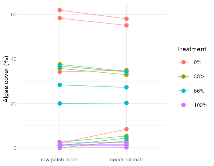
A random effect does not just adjust the p-value. It changes each patch’s estimate.

Note

📖 New word: shrinkage

Every patch estimate is pulled toward its treatment mean. The model treats an extreme patch average as partly real signal and partly luck, and splits the difference.

Patches with fewer quadrats, or more internal scatter, get pulled further.

Tip

🖐 Why this is a feature

A patch whose 5 quadrats happened to land high is probably not that extreme — the next 5 would come back closer to average. Shrinkage builds that expectation in, instead of taking every noisy group mean at face value.

This is called partial pooling: somewhere between treating every patch as unrelated and pretending they are all identical.

Mixed-Model ANOVA — Method 1: F-Distribution

• Accounts for the uncertainty in variance-component estimation
• More conservative (higher p-values)
• Better for small samples

# car::Anova uses Kenward-Roger denominator df for test.statistic = "F"
# (that is what the printed header says -- there is no ddf argument here)
u_anova_result <- Anova(u_lmer_model, type = 3, test.statistic = "F")
cat("Type III ANOVA with F test:\n\n")
## Type III ANOVA with F test:
u_anova_result
## Analysis of Deviance Table (Type III Wald F tests with Kenward-Roger df)
## 
## Response: algae
##                   F Df Df.res   Pr(>F)   
## (Intercept) 18.5551  1     12 0.001018 **
## treat        2.7171  3     12 0.091262 . 
## ---
## Signif. codes:  0 '***' 0.001 '**' 0.01 '*' 0.05 '.' 0.1 ' ' 1

Mixed-Model ANOVA — Method 2: Chi-Square

• Assumes variance components are known (not estimated)
• More liberal (lower p-values)
• Assumes large samples

Why different results? Chi-square = F × numerator df. The F-test accounts for the denominator df (12, here — reflecting sample size); Chi-square assumes infinite denominator df (i.e., a large sample).

Rule of thumb: under 100 observations or < 20 random-effect levels, use the F-test. Over 500 observations and > 50 random-effect levels, Chi-square is okay. In between, the F-test is safer.

u_anova_chisq <- Anova(u_lmer_model, type = 3, test.statistic = "Chisq")
cat("Type III ANOVA with Chi-square test:\n\n")
## Type III ANOVA with Chi-square test:
u_anova_chisq
## Analysis of Deviance Table (Type III Wald chisquare tests)
## 
## Response: algae
##               Chisq Df Pr(>Chisq)    
## (Intercept) 18.5551  1 0.00001651 ***
## treat        8.1513  3    0.04299 *  
## ---
## Signif. codes:  0 '***' 0.001 '**' 0.01 '*' 0.05 '.' 0.1 ' ' 1

The Nested Model, Restated

\[algae_{ijk} = \mu + \alpha_i + \beta_{j(i)} + \epsilon_{ijk}\]

• \(\mu\) is the overall mean
• \(\alpha_i\) is the fixed effect of treatment i
• \(\beta_{j(i)}\) is the random effect of patch j nested within treatment i
• \(\epsilon_{ijk}\) is the residual error for quadrat k in patch j within treatment i

## Final ANOVA results:
## Analysis of Deviance Table (Type III Wald F tests with Kenward-Roger df)
## 
## Response: algae
##                   F Df Df.res   Pr(>F)   
## (Intercept) 18.5551  1     12 0.001018 **
## treat        2.7171  3     12 0.091262 . 
## ---
## Signif. codes:  0 '***' 0.001 '**' 0.01 '*' 0.05 '.' 0.1 ' ' 1

Part 3 · Post-Hoc and Interpretation

Interpreting the Variance Components

Important

⚠️ Two tests, two answers — and you must pick one before you look

Test	Statistic	p	Verdict at α = 0.05
F (Kenward-Roger df)	F₃,₁₂ = 2.72	0.091	not significant
Wald χ²	χ² = 8.15	0.043	significant

Same model. Same data. Opposite conclusions.

The χ² test assumes it knows the variance components exactly and that the sample is large. We have 16 patches. It is being over-confident, exactly as the rule of thumb two slides back predicted.

Report the F-test. It agrees with last week’s aov(Error(patch)) result to four decimal places — because it is the same test.

Note

How to report this result

“Algal cover did not differ significantly among urchin density treatments (linear mixed model with patch as a random effect, F₃,₁₂ = 2.72, p = 0.091, Kenward-Roger denominator df). Among-patch variance was substantial (σ²_patch = 294.3 vs σ²_residual = 298.6, ICC = 0.50), indicating strong spatial heterogeneity in algal cover.”

Post-Hoc Comparisons

Although the main effect of treatment was marginally significant (p = 0.04306), we can examine mean differences between treatments to understand patterns in the data.

u_emm <- emmeans(u_lmer_model, ~ treat)
cat("Estimated marginal means:\n\n")
## Estimated marginal means:
u_emm
##  treat emmean   SE df lower.CL upper.CL
##  0%      39.2 9.41 12    18.70     59.7
##  33%     19.0 9.41 12    -1.50     39.5
##  66%     21.6 9.41 12     1.05     42.0
##  100%     1.3 9.41 12   -19.20     21.8
## 
## Degrees-of-freedom method: kenward-roger 
## Confidence level used: 0.95

u_pairs <- pairs(u_emm, adjust = "sidak")
cat("Pairwise comparisons (Sidak adjusted):\n\n")
## Pairwise comparisons (Sidak adjusted):
u_pairs
##  contrast   estimate   SE df t.ratio p.value
##  0% - 33%      20.20 13.3 12   1.518  0.6356
##  0% - 66%      17.65 13.3 12   1.327  0.7557
##  0% - 100%     37.90 13.3 12   2.849  0.0848
##  33% - 66%     -2.55 13.3 12  -0.192  1.0000
##  33% - 100%    17.70 13.3 12   1.330  0.7534
##  66% - 100%    20.25 13.3 12   1.522  0.6331
## 
## Degrees-of-freedom method: kenward-roger 
## P value adjustment: sidak method for 6 tests

Compact Letter Display

u_cld <- multcomp::cld(u_emm, alpha = 0.05, Letters = letters)
cat("Compact letter display:\n\n")
## Compact letter display:
u_cld
##  treat emmean   SE df lower.CL upper.CL .group
##  100%     1.3 9.41 12   -19.20     21.8  a    
##  33%     19.0 9.41 12    -1.50     39.5  a    
##  66%     21.6 9.41 12     1.05     42.0  a    
##  0%      39.2 9.41 12    18.70     59.7  a    
## 
## Degrees-of-freedom method: kenward-roger 
## Confidence level used: 0.95 
## P value adjustment: tukey method for comparing a family of 4 estimates 
## significance level used: alpha = 0.05 
## NOTE: If two or more means share the same grouping symbol,
##       then we cannot show them to be different.
##       But we also did not show them to be the same.

Important

Interpreting treatment comparisons

Mean algae cover shows a pattern with increasing urchin density: None/Removed (39.20%) > Medium/33% Density (19.00%) > High/66% Density (21.55%) > Low/Control (1.30%). This suggests an inverse relationship between urchin density and algae cover. The high variability among patches within treatments contributed to the marginal statistical significance for the treatment effect.

Part 4 · Assumptions and Visualization

ANOVA Assumptions Testing — Base R

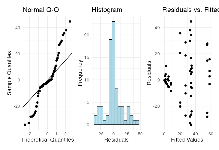
For valid inference from ANOVA, several assumptions must be met. We test these below with a base R approach — note that it doesn’t work all that well for a mixed model.

Tip

🖐 Notice

plot(mixed_model) and friends were built for lm() objects — they mostly work for lmer(), but purpose-built tools like DHARMa do a better job (see the Nested ANOVA activity).

Diagnostic Plots

Levene’s Test for Homogeneity of Variance

u_levene <- leveneTest(algae ~ treat, data = u_df)
cat("Levene's test for homogeneity of variance:\n\n")
## Levene's test for homogeneity of variance:
u_levene
## Levene's Test for Homogeneity of Variance (center = median)
##       Df F value     Pr(>F)    
## group  3  8.1694 0.00008785 ***
##       76                       
## ---
## Signif. codes:  0 '***' 0.001 '**' 0.01 '*' 0.05 '.' 0.1 ' ' 1

Important

Interpreting the assumption tests

The Q-Q plot shows some deviation from normality, particularly in the tails, and Levene’s test indicates significant heterogeneity of variances across treatments (p = 0.00008785). Quinn & Keough (2002) noted “large differences in within-cell variances” in this dataset, and transformations (including arcsin) did not improve variance homogeneity. However, ANOVA is generally robust to heteroscedasticity with balanced designs, which is why they analyzed untransformed data. The Residuals vs. fitted plot also shows a pattern of increasing variance with increasing fitted values, confirming the heteroscedasticity.

Visualization — Boxplot

Visualization — Means Plot

Part 5 · Discussion and Manual Calculation

Scientific Interpretation

Important

Our mixed-model analysis revealed substantial spatial heterogeneity in algae cover, with significant variation among patches within each treatment. The effect of urchin density treatments on filamentous algae cover was marginally significant at the α = 0.05 level (p = 0.043). Descriptive statistics show algae cover increasing as urchin density decreases, with None/Removed showing the highest cover (39.20%), followed by Medium/33% Density (19.00%), High/66% Density (21.55%), and Low/Control showing minimal algae cover (1.30%). The variance component for patches nested within treatments (294.31, ~39.5% of total variance) shows that spatial heterogeneity is a major structuring force in these algal communities, and needs to be accounted for when designing and analyzing ecological field experiments.

We Can Do This Manually — but Ugh

Nobody would ever do this by hand in practice — but seeing it once makes the “which MS goes on the bottom of the F-ratio” logic concrete, and shows how the traditional nested-ANOVA F-ratio (last lecture) connects to the mixed-model result above.

u_man_model <- aov(algae ~ treat + treat:patch, data = u_df)
u_anova_summary <- summary(u_man_model)[[1]]
cat("Standard ANOVA table:\n\n")
## Standard ANOVA table:
u_anova_summary
##             Df Sum Sq Mean Sq F value        Pr(>F)    
## treat        3  14429  4809.7 16.1075 0.00000006579 ***
## treat:patch 12  21242  1770.2  5.9282 0.00000083226 ***
## Residuals   64  19110   298.6                          
## ---
## Signif. codes:  0 '***' 0.001 '**' 0.01 '*' 0.05 '.' 0.1 ' ' 1

u_MS_treat <- u_anova_summary[1, "Mean Sq"]
u_MS_patch <- u_anova_summary[2, "Mean Sq"]
u_MS_residual <- u_anova_summary[3, "Mean Sq"]

u_df_treat <- u_anova_summary[1, "Df"]
u_df_patch <- u_anova_summary[2, "Df"]
u_df_residual <- u_anova_summary[3, "Df"]

cat("MS Treatment:", u_MS_treat, "\n")
## MS Treatment: 4809.712
cat("MS Patch(Treatment):", u_MS_patch, "\n")
## MS Patch(Treatment): 1770.163
cat("MS Residual:", u_MS_residual, "\n\n")
## MS Residual: 298.6

u_F_treat_correct <- u_MS_treat / u_MS_patch        # Treatment tested against patches
u_F_patch <- u_MS_patch / u_MS_residual             # Patches tested against residual

cat("F Treatment:", u_F_treat_correct, "\n")
## F Treatment: 2.717102
cat("F Patch(Treatment):", u_F_patch, "\n\n")
## F Patch(Treatment): 5.928207

u_p_treat_correct <- pf(u_F_treat_correct, u_df_treat, u_df_patch, lower.tail = FALSE)
u_p_patch <- pf(u_F_patch, u_df_patch, u_df_residual, lower.tail = FALSE)

u_corrected_table <- data.frame(
  Source = c("Treatment", "Patches(Treatment)", "Residual"),
  Df = c(u_df_treat, u_df_patch, u_df_residual),
  MS = round(c(u_MS_treat, u_MS_patch, u_MS_residual), 1),
  F = c(round(u_F_treat_correct, 2), round(u_F_patch, 2), NA),
  p = c(ifelse(u_p_treat_correct < 0.001, "<0.001", round(u_p_treat_correct, 3)),
        ifelse(u_p_patch < 0.001, "<0.001", round(u_p_patch, 3)),
        NA)
)
cat("Corrected ANOVA table:\n\n")
## Corrected ANOVA table:
u_corrected_table
##               Source Df     MS    F      p
## 1          Treatment  3 4809.7 2.72  0.091
## 2 Patches(Treatment) 12 1770.2 5.93 <0.001
## 3           Residual 64  298.6   NA   <NA>

The lmer Formula Cheat-Sheet

Read every random term as ( what varies | across what ).

Formula	Meaning
y ~ x + (1|g)	random intercept per group — each group has its own baseline
y ~ x + (1 + x|g)	random intercept and slope — each group has its own baseline and its own response to x
y ~ x + (0 + x|g)	random slope only, shared intercept
y ~ x + (1|a) + (1|b)	two crossed random factors
y ~ x + (1|a/b)	b nested in a — shorthand for (1|a) + (1|a:b)

Important

⚠️ The confusion to avoid

(1|patch) and (1|treat:patch) are both random-intercept models. The 1 is the intercept; what differs is only the grouping.

You only have a random slope when something other than 1 appears on the left of the |.

Tip

🖐 Do I need a/b here?

Only if the inner IDs restart inside each outer level (patch 1,2,3,4 in every treatment). Then R cannot tell nesting from crossing and you must write (1|treat/patch).

Our patches are numbered 1–16 across the whole study, so (1|patch) already says it.

Warning

⚠️ “boundary (singular) fit”

Means a variance was estimated as ~0 — the grouping factor explains nothing, or you asked for more random structure than the data can support. Simplify the random effects; do not ignore it.

Wrap-up

Today you:

• Decided fixed vs random by asking whether you care about these levels or about how much they vary
• Learned that a random factor costs one parameter (a variance) where a fixed one costs k − 1
• Read (1|group) correctly, and saw that it is not a random slope
• Got the ICC = 0.50 — two quadrats in a patch are half-correlated, which is exactly why this design needed a mixed model
• Saw partial pooling move each patch estimate toward its treatment mean
• Chose between the F-test (p = 0.091) and the Wald χ² (p = 0.043) — and learned why the F-test is the right one at n = 16 groups

Important

⚠️ Report the F-test, and say so

With few random-effect levels the χ² is anti-conservative — it assumes it knows the variance components exactly. Always state which approximation you used and what the denominator df were.

Note

✅ The one idea to keep

A mixed model does not “remove” the patch effect — it estimates it, and then tests the treatment against the right amount of noise.

σ²_patch = 294.3 arrived three ways: by hand from mean squares, from aov(Error(patch)), and from VarCorr(). Same model, three notations. If you understood the nested ANOVA, you already understood mixed models — this is just a better way to write and fit them.

Tip

🖐 Before next class

Take the pine needle data, collapsed to one value per team per side (the two-stage summary from Week 3):

p_df <- pine_df |>
  group_by(team, side) |>
  summarise(needle_length_mm = mean(needle_length_mm),
            .groups = "drop")

anova(lmer(needle_length_mm ~ side + (1|team), data = p_df))

Compare F to the square of the paired-t statistic from Week 4 (t = −2.72). You should get F = 7.41, df 1 and 3, p = 0.072 — the paired t-test is this mixed model.

🚀 If you finish early: run the same formula on the raw 64 needles instead. You get p = 0.057 and 59 denominator df, not 3. What changed? (Hint: check VarCorr() — one variance is estimated as exactly zero, and R warns “singular fit”.)

Getting unstuck

When code breaks — and it will, that is normal:

1. Read the error message out loud; it usually names the line
2. Check the usual suspects: is the grouping variable a factor? Is lmerTest loaded (plain lme4 gives no p-values on purpose)? Are you calling car::Anova() on the model rather than anova()?
3. “boundary (singular) fit” → your random structure is too complex for the data, or that variance really is zero
4. “Model failed to converge” → try control = lmerControl(optimizer = "bobyqa"), as we did here, or simplify the random effects
5. Bring the exact error (copy-paste it) to class or office hours

Note

✅ Key idea

Every working scientist googles error messages daily. Getting stuck is not failing — it is the job.