## Data
## # A tibble: 6 × 4
##   treat patch  quad algae
##   <fct> <fct> <dbl> <dbl>
## 1 100%  1         1     0
## 2 100%  1         2     0
## 3 100%  1         3     0
## 4 100%  1         4     6
## 5 100%  1         5     2
## 6 100%  2         1     0
##
##
## Treatment levels:
## [1] "0%" "33%" "66%" "100%"Lecture: Nested ANOVA
Hierarchical designs
ANOVA
Factorial vs. nested designs, the nested-ANOVA linear model and variance partitioning, and a naive-vs-correct worked example (sea urchin grazing and algae cover) using the traditional aov() approach — the modern mixed-model (lmer) alternative continues in the Linear Mixed Models lecture.
Where We Left Off
Covered last time — two-factor ANOVA:
- Example, linear model, analysis of variance
- Null hypotheses
- Interactions and main effects
- Unequal sample size
- Assumptions
Note
✅ Key idea from last lecture
In a factorial design, every level of B appears under every level of A. Today: what happens when B is only ever nested inside one specific level of A?
Part 1 · Multifactor Designs
Two-Factor (2-Way) ANOVA, Recap
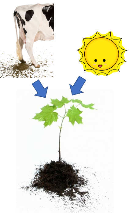
- We often consider more than 1 factor (independent categorical variables) to reduce unexplained variance and look at interactions
- 2-factor designs (2-way ANOVA) are very common in ecology
- Can have more factors (e.g., 3-way ANOVA) — interpretation gets tricky
- Most multifactor designs are: factorial, nested, or mixed
Factorial Versus Nested Designs
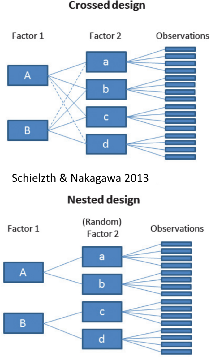
Consider two factors, A and B:
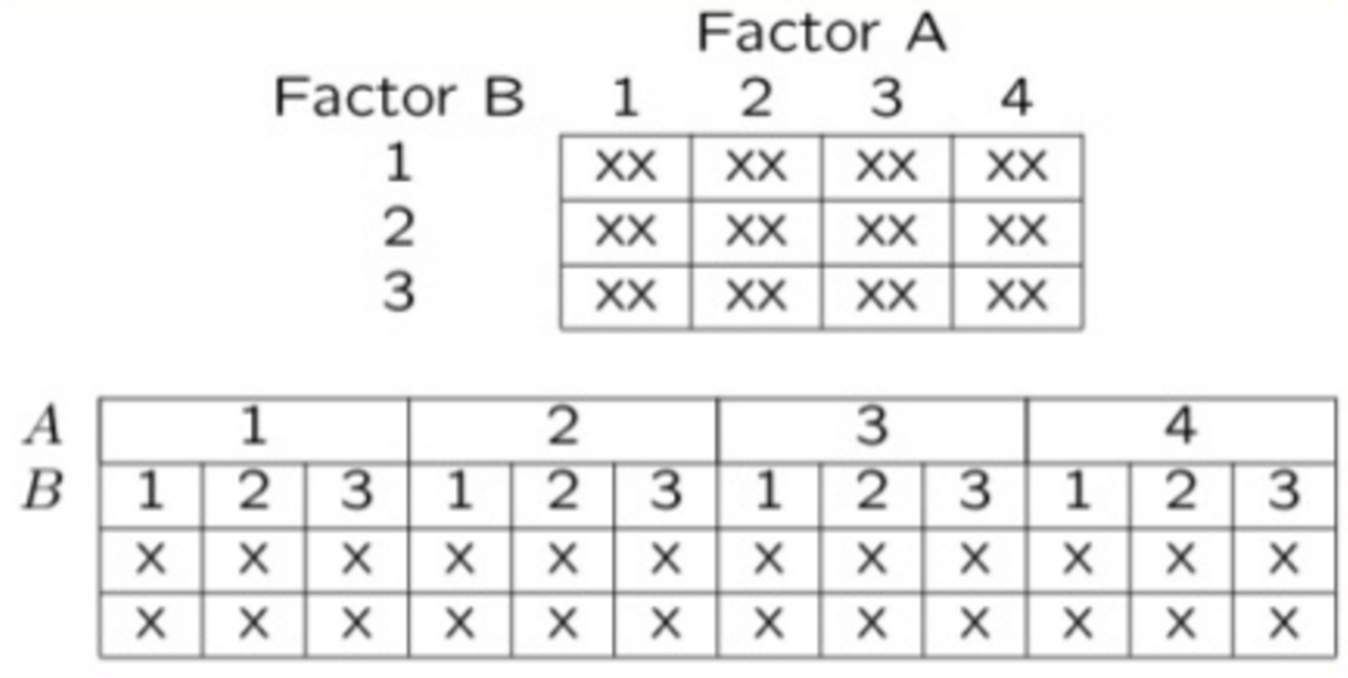
- Factorial/crossed: every level of B in every level of A
- Nested/hierarchical: levels of B occur only in 1 level of A
- both fixed — rare
- one fixed, one random
- both random — rare in ecology, common in genetics
Part 2 · Factorial Designs — Examples
Factorial Designs Overview
Factorial designs: both factors are typically fixed (but not always).
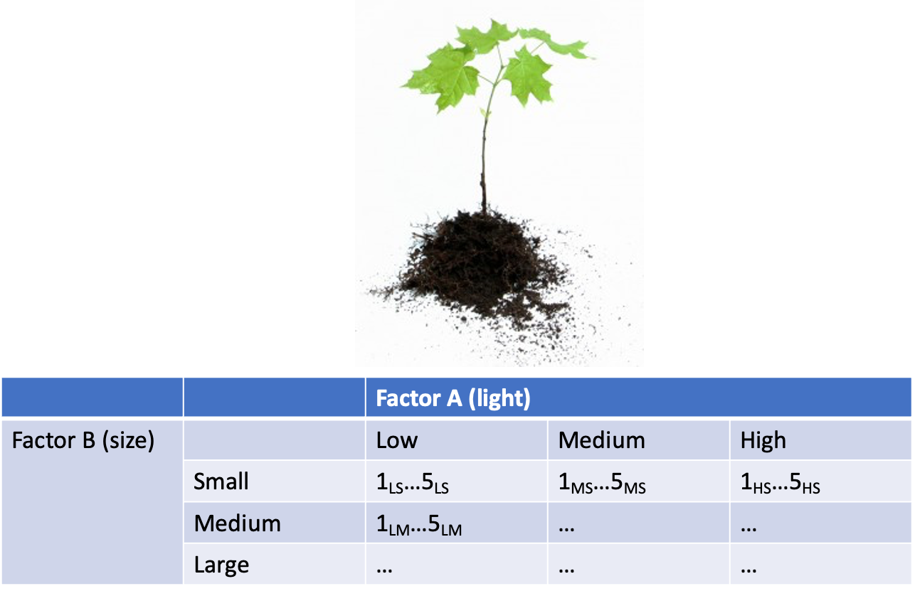
Factorial Design Example: Seedling Growth
Effects of light level on growth of seedlings of different size:
- 3 light levels (Factor A)
- 3 size classes (Factor B)
- 5 replicate seedlings in each cell
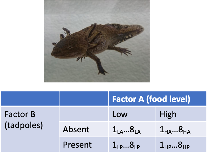
Factorial Design Example: Salamander Growth
Effects of food level and tadpole presence on larval salamander growth:
- 2 food levels (Factor A)
- Presence/absence of tadpoles (Factor B)
- 8 replicates in each cell
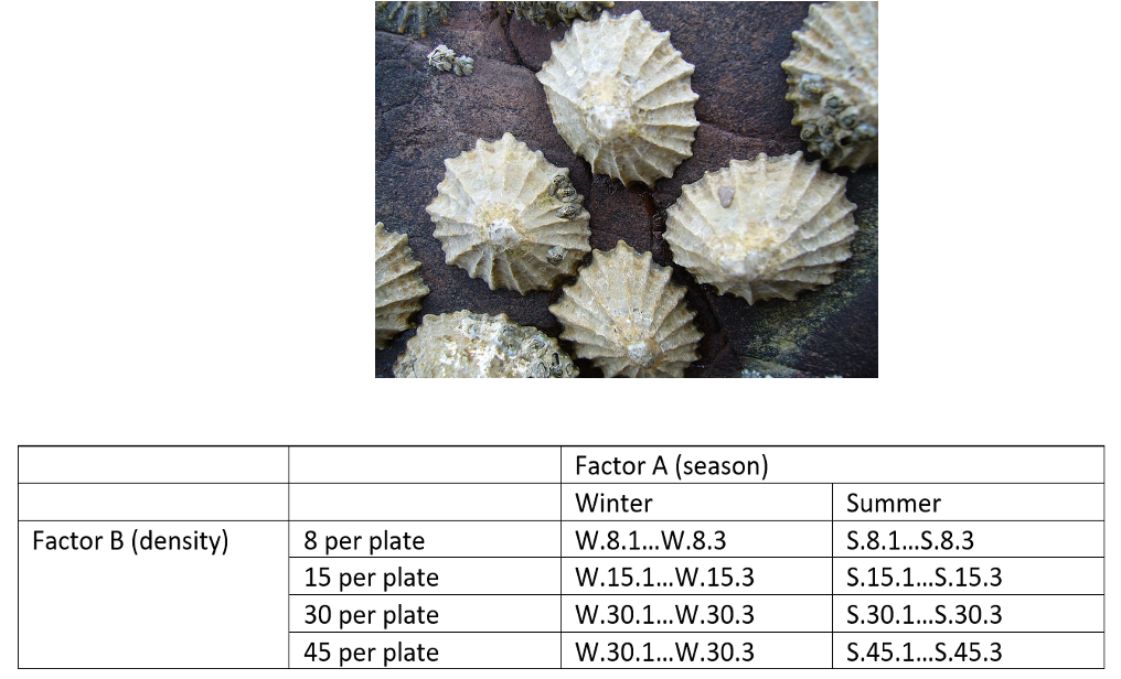
Factorial Design Example: Limpet Fecundity
Effect of season and density on limpet fecundity:
- 2 seasons (Factor A)
- 4 density treatments (Factor B)
- 3 replicates in each cell
Part 3 · Nested Designs — Examples
Nested Designs Overview
Nested designs cover: nested design examples, the linear model, analysis of variance, null hypotheses, unbalanced designs, assumptions, mixed-model ANOVA.
Nested designs: Factor A is usually fixed; Factor B is usually random.

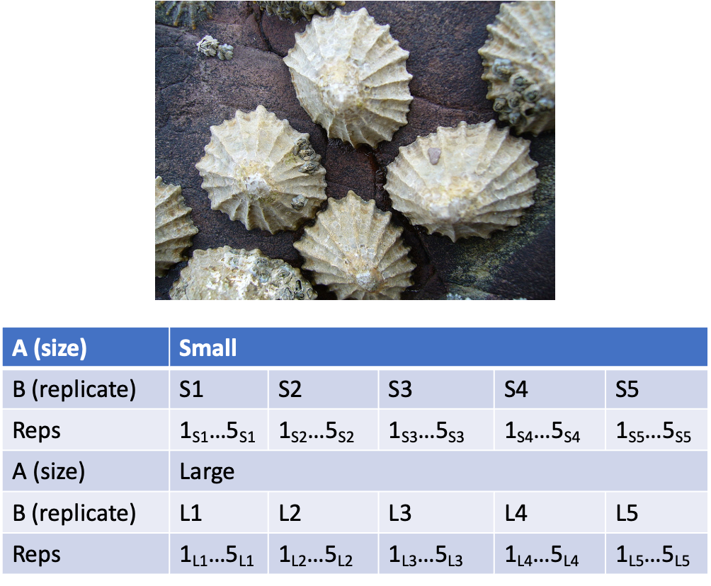
Nested Design Example: Limpet Growth
Study on effects of enclosure size on limpet growth:
- 2 enclosure sizes (Factor A)
- 5 replicate enclosures (Factor B)
- 5 replicate limpets per enclosure
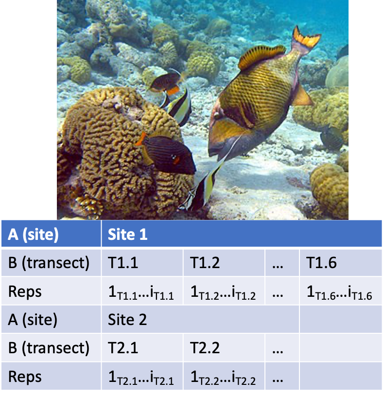
Nested Design Example: Reef Fish
Study on reef fish recruitment:
- 5 sites (Factor A)
- 6 transects at each site (Factor B)
- Replicate observations along each transect
Nested Design Example: Sea Urchin Grazing
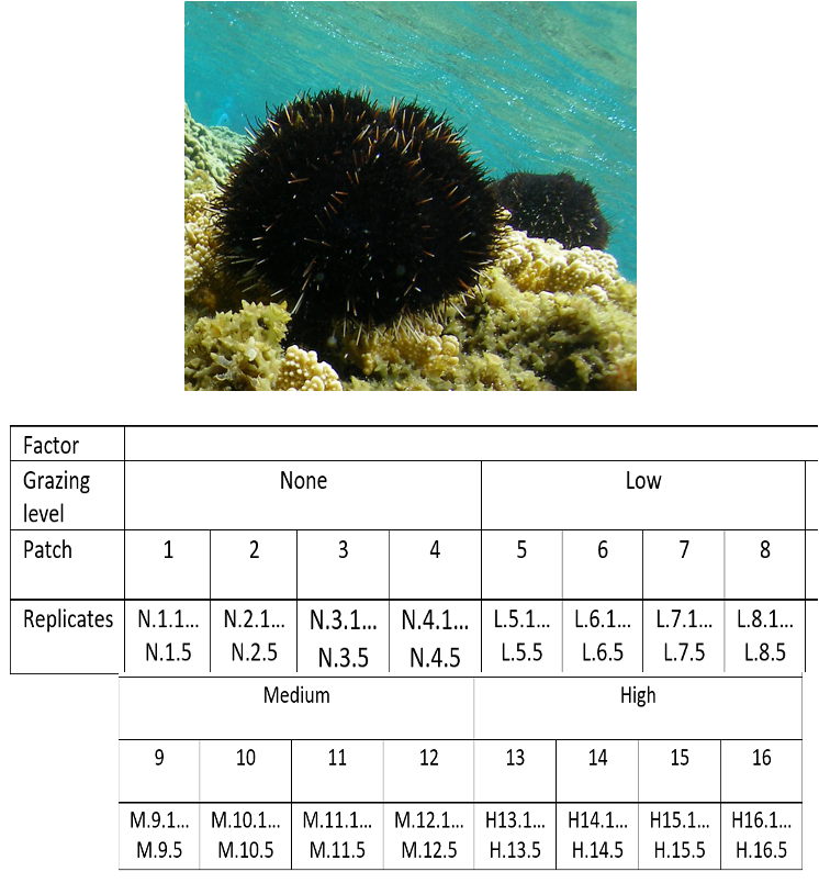
Effects of sea urchin grazing on biomass of filamentous algae:
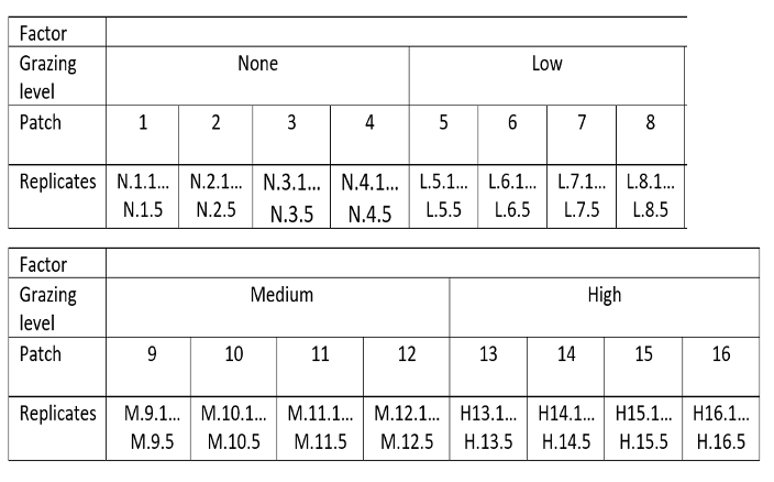
- 4 urchin densities: 0%, 33%, 66%, 100% of natural density
- 4 patches of rocky bottom (3–4 m²) nested in each grazing level
- 5 replicate quadrats per patch
This is our worked example for the rest of the lecture.
Part 4 · The Nested Design Model
Nested Design: Linear Model Structure
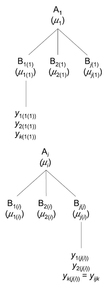
Consider a nested design with:
- p levels of factor A (i = 1…p) — e.g., 4 grazing levels
- q levels of factor B (j = 1…q), nested within each level of A — e.g., 4 different patches per grazing level
- n replicates (k = 1…n) in each combination of A and B — e.g., 5 replicate quadrats in each patch in each grazing level
Calculating Means in a Nested Design
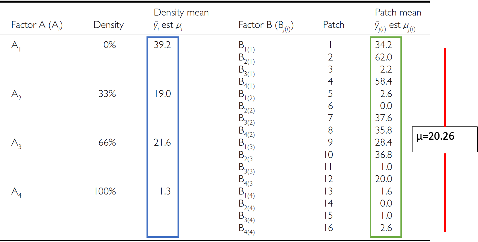
We can calculate several means:
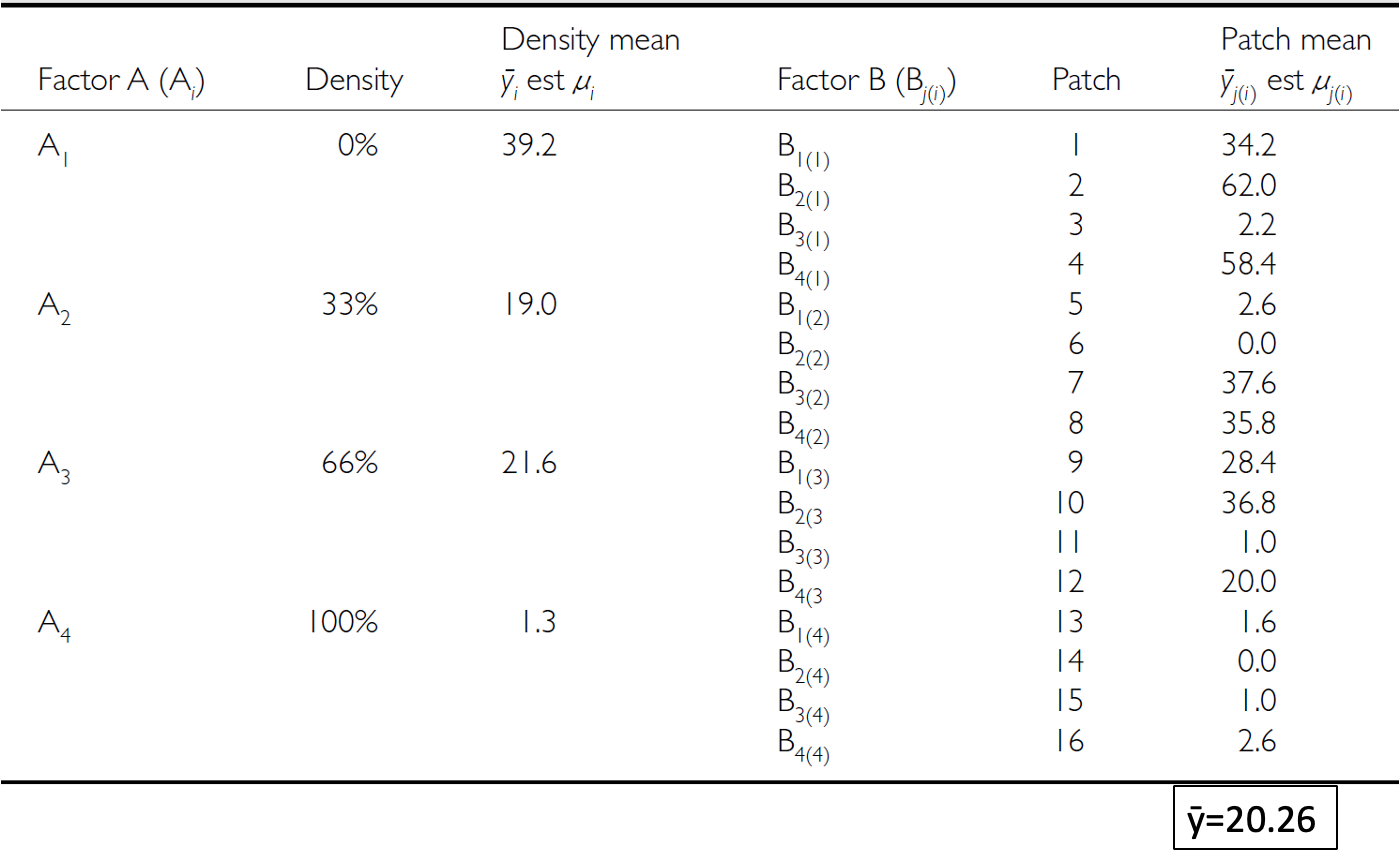
- Overall mean (across all levels of A and B) = \(\bar{y}\)
- A mean for each level of A (across all levels of B in that A) = \(\bar{y}_i\)
- A mean for each level of B within each A = \(\bar{y}_{j(i)}\)
Nested Design Means, Visualized
The Nested Design Linear Model
\[y_{ijk} = \mu + \alpha_i + \beta_{j(i)} + \varepsilon_{ijk}\]
- \(y_{ijk}\) is the response variable — the value of the k-th replicate in the j-th level of B in the i-th level of A (e.g., algal biomass in the 3rd quadrat, in the 2nd patch, in the low-grazing treatment)
- \(\mu\) is the overall mean (overall average algal biomass)
Tip
🖐 Notice
This looks almost identical to the two-way ANOVA model — the difference is entirely in the subscript: \(\beta_{j(i)}\), not \(\beta_j\). B only exists inside a specific A.
Fixed and Random Effects in the Nested Model
\[y_{ijk} = \mu + \alpha_i + \beta_{j(i)} + \varepsilon_{ijk}\]
- \(\alpha_i\) is the fixed effect of factor A — the difference between the average biomass in all low-grazing-level quadrats and the overall mean
- \(\beta_{j(i)}\) is the random effect of factor B nested within factor A — usually a random variable measuring variance among all possible levels of B within each level of A (variance among all possible patches that could have been used in the low-grazing treatment)
Note
✅ Key idea
B being random is the whole point of nesting: you don’t care about these specific patches — you care about patch-to-patch variability in general.
The Error Term in the Nested Model
\[y_{ijk} = \mu + \alpha_i + \beta_{j(i)} + \varepsilon_{ijk}\]
- \(\varepsilon_{ijk}\) is the error term — the unexplained variance associated with the k-th replicate in the j-th level of B in the i-th level of A
- \(\alpha_i\) is the effect of the i-th level of A: \(\mu_i - \mu\)
- \(\varepsilon_{ijk}\): the difference between the observed algal biomass in the 3rd quadrat in the 2nd patch in the low-grazing treatment, and the predicted biomass (the average biomass in that 2nd patch in the low-grazing treatment)
Tip
🖐 Notice
The residual is measured against the cell mean (this specific patch), not the treatment mean — that’s what makes it “nested,” arithmetically.
Part 5 · Partitioning Variance
Analysis of Variance: Residual and Total
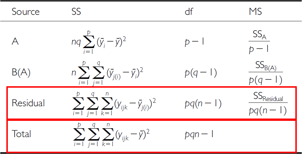
- \(SS_{resid}\) is the difference between each observation and the mean for its level of factor B, summed over all observations
- \(SS_{total} = SS_A + SS_B + SS_{resid}\)
- SS can be turned into MS by dividing by the appropriate df
Analysis of Variance: SSA
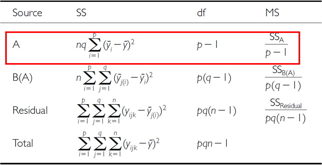
As before, we partition the variance in the response variable using SS. \(SS_A\) is the SS of differences between the mean in each level of A and the overall mean.
Analysis of Variance: SSB
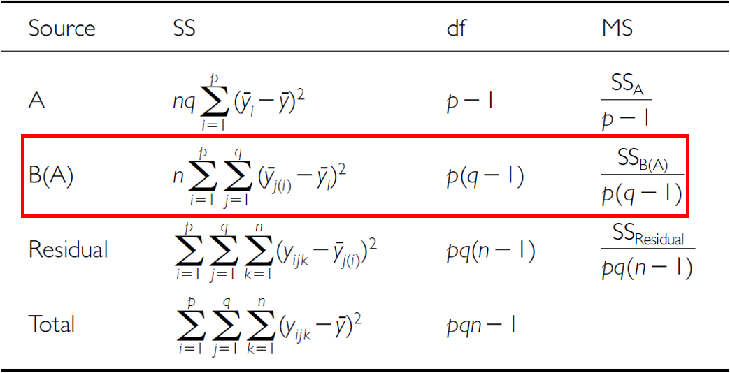
\(SS_B\) is the SS of the difference between the mean in each level of B and the mean of the corresponding level of A, summed across all levels of A.
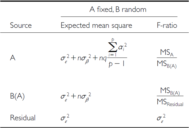
The Nested ANOVA Table
Part 6 · Hypotheses and Assumptions
Null Hypotheses: Factor A
Two hypotheses are tested on values of MS. 1. No effects of factor A — assuming A is fixed:
- \(H_0(A)\): \(\mu_1 = \mu_2 = ... = \mu_i = \mu\)
- Same as in 1-factor ANOVA, using means from B factors nested within each level of A
- (no difference in algal biomass across all grazing levels: \(\mu_{none} = \mu_{low} = \mu_{med} = \mu_{high}\))
Null Hypotheses: Factor B
2. No effects of factor B nested in A — assuming B is random:
- \(H_0(B)\): \(\sigma^2_\beta = 0\) (no variance added due to differences between all possible levels of B)
- (no variance added due to differences between patches)
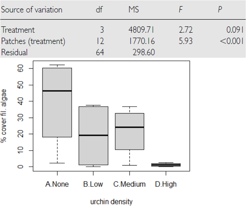
Conclusions from the Analysis
Conclusion:
“Significant variation between replicate patches within each treatment, but no significant difference in the amount of filamentous algae between treatments.”
Unbalanced Nested Designs
Unequal sample sizes can arise from:
- An uneven number of B levels within each A
- An uneven number of replicates within each level of B
Not a problem unless you have unequal variance or a large deviation from normality.
Nested Design Assumptions
As usual, we assume: equal variance, normality, no outliers, independence of observations.
Equal variance + normality need to be assessed at both levels:
- Since means for each level of B within each A are used for the H-test about A, need to assess whether those means meet normality and equal variance
- Examine residuals for the H-test about B
- Transformations can be used
Warning
⚠️ Watch out!
This is the part people most often get wrong: checking assumptions on the raw data isn’t enough for a nested design — you need to check them at the level each hypothesis test actually operates on.
Part 7 · The Sea Urchin Example — Data
The Nested Design, the Hard Way
This analysis examines the effects of varying sea urchin densities on the percentage cover of filamentous algae. The experiment was designed with:
- Four random patches
- Four urchin density treatments — 0% (urchins removed), 33%, 66%, and 100% of natural density (the unmanipulated control)
- Five replicate quadrats measured within each treatment-patch combination
Note
📖 Reference
Quinn & Keough (2002), Experimental Design and Data Analysis for Biologists — this dataset and analysis follow their treatment of the sea urchin/algae example.
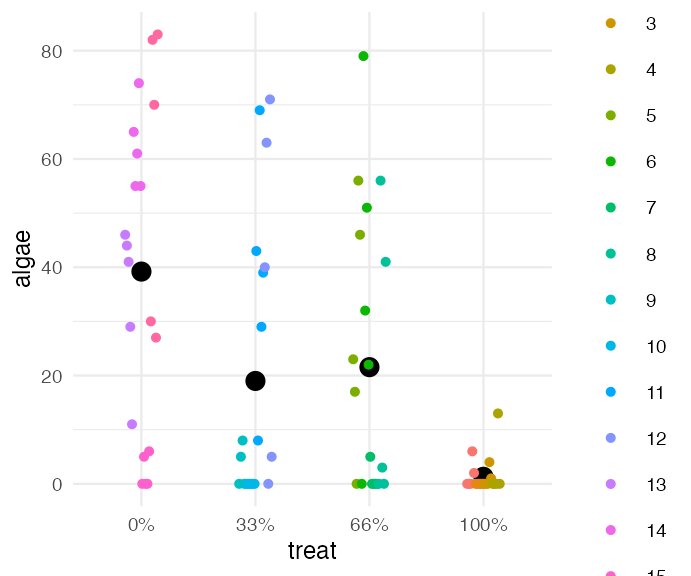
Data Overview
The data frame contains: patch (random patches 1–16 where treatments were applied), treat (urchin density treatment), quad (replicate quadrats within each treatment-patch combination), algae (percentage cover of filamentous algae — the response variable).
## Summary statistics by treatment:
## # A tibble: 4 × 7
##   treat     n  mean    sd    se   min   max
##   <fct> <int> <dbl> <dbl> <dbl> <dbl> <dbl>
## 1 0%       20  39.2 28.7  6.41      0    83
## 2 33%      20  19   25.7  5.74      0    71
## 3 66%      20  21.6 25.1  5.62      0    79
## 4 100%     20   1.3  3.18 0.711     0    13
A First Look at the Data
Part 8 · The Wrong Way — Naive Factorial Model
Manual Nested ANOVA — Setting Up
In this experimental design, patch is nested within treat because each patch received only one treatment level — a hierarchical design where the effect of patches must be considered within each treatment (Quinn & Keough 2002).
We’ll use a traditional nested ANOVA. You could make this easy by averaging algae per patch and running a one-way ANOVA — but your power is significantly reduced, and you lose estimates of variability among patches.
This first attempt is really a regular factorial ANOVA — not appropriate, since it’s pseudoreplicated. Also, the F-value for Treat is using \(MS_{resid}\) when it should use \(MS_{treat:patch}\).
u_fact_model <- aov(algae ~ treat + treat:patch, data = u_df)
cat("Factorial model summary:\n\n")
## Factorial model summary:
summary(u_fact_model)
##             Df Sum Sq Mean Sq F value       Pr(>F)
## treat        3  14429    4810  16.108 0.0000000658 ***
## treat:patch 12  21242    1770   5.928 0.0000008323 ***
## Residuals   64  19110     299
## ---
## Signif. codes:  0 '***' 0.001 '**' 0.01 '*' 0.05 '.' 0.1 ' ' 1
Why the Factorial ANOVA Is Not Correct
- We can correct this by specifying the error term
- The MS needed for the F-value is really MS(patch nested in treatment), because those are the true replicates
- We can specify that — the problem is this approach can’t really handle unbalanced designs
# Error(patch) -- not Error(treat:patch). Patch IDs are already unique
# (1-16) and each patch sits in exactly one treatment, so naming the patch
# alone is enough. Writing treat:patch asks for 4 x 16 = 64 combinations
# when only 16 exist, which makes R warn "Error() model is singular".
# Both give identical numbers; this one does it without the warning.
u_nested_model <- aov(algae ~ treat + Error(patch), data = u_df)
cat("Correctly specified nested ANOVA:\n\n")
## Correctly specified nested ANOVA:
summary(u_nested_model)
##
## Error: patch
##           Df Sum Sq Mean Sq F value Pr(>F)
## treat      3  14429    4810   2.717 0.0913 .
## Residuals 12  21242    1770
## ---
## Signif. codes:  0 '***' 0.001 '**' 0.01 '*' 0.05 '.' 0.1 ' ' 1
##
## Error: Within
##           Df Sum Sq Mean Sq F value Pr(>F)
## Residuals 64  19110   298.6
Same Numerator, Different Denominator
Both models used the same 80 quadrats and produced the same sums of squares. Only the F-test’s denominator changed:
| MS treat | ÷ MS error | = F | p | |
|---|---|---|---|---|
| Naive factorial | 4810 | ÷ 299 (quadrats) | 16.11 | 0.00000007 |
| Nested | 4810 | ÷ 1770 (patches) | 2.72 | 0.091 |
Important
The p-value moved by six orders of magnitude.
The naive model tested the treatment against variation between quadrats within a patch — but quadrats are not what we assigned treatments to. Patches are.
There are 80 quadrats but only 16 patches, four per treatment. The honest test has 12 denominator degrees of freedom, not 64.
Note
✅ How to find the right denominator
Ask: what did I randomly assign the treatment to?
That unit — patch here — supplies the error term. Everything measured inside it is a subsample, and subsamples tell you about measurement noise, not about treatment effects.
Tip
🖐 Notice MS(patch) is large
1770 vs 299 — patches genuinely differ from one another. That variability is real biology, and the nested model makes you pay for it. The naive model pretended it was not there.
Where You Have Seen This Before
This is the pine needle problem again, one level up:
| Our pine study | This urchin study |
|---|---|
| 8 needles per side | 5 quadrats per patch |
| within one tree | within one patch |
| 4 trees are the replicates | 16 patches are the replicates |
| 64 rows, n = 4 | 80 rows, n = 16 |
In Week 1 we solved it by averaging each tree to one number. That works, and it is honest.
A nested ANOVA does something better: it keeps every quadrat, estimates both levels of variability, and still tests the treatment against the right error term.
Note
✅ Key idea
Averaging throws the subsamples away. Nesting uses them — to estimate how noisy your measurements are — while still refusing to count them as replicates.
Warning
⚠️ The limit of aov(Error(...))
This syntax needs a (near-)balanced design. Ours is perfectly balanced — 4 patches per treatment, 5 quadrats per patch — so it works.
Real data usually is not. That is the problem mixed models solve, and it is where we go next.
How Do I Know If My Design Is Nested?
Three questions, in order. Ask them of your own data before you fit anything.
1. What did I apply the treatment to? → Whole patches. Not quadrats.
2. Does every level of B appear under every level of A? → Patch 7 only ever received the 66% density. It cannot appear under 100%. → No ⇒ nested. (Yes ⇒ crossed/factorial.)
3. How many of those units do I have per treatment? → 4 patches, not 20 quadrats. That is your n.
Important
The answer to Q1 is your error term.
aov(algae ~ treat + Error(patch), data = u_df)
#                   ^^^^^^^^^^^^
#                   the thing treatments were assigned to
Tip
🖐 A quick tell
If two rows of your data share a value for the thing you randomized, they are not independent replicates of it.
Two quadrats in patch 3 share patch 3. Two needles on one tree share that tree.
Warning
⚠️ Nested factors are random
We are not asking “is patch 7 different from patch 12?” — those specific patches are of no interest. They are a sample of possible patches, so patch enters as a random effect.
The factor above it (treat) is fixed: those four densities are exactly the ones we care about.
Reporting a Nested ANOVA
Note
How to report this result
“Algal cover did not differ significantly among urchin density treatments (nested ANOVA, F₃,₁₂ = 2.72, p = 0.091), with patches treated as a random factor nested within treatment. Variation among patches within treatments was substantial, accounting for approximately 50% of the total variance (σ²_patch = 294, σ²_within = 299; n = 4 patches per treatment, 5 quadrats per patch).”
The three things people get wrong:
- The degrees of freedom. It is F(3, 12) — the denominator df comes from the patch stratum, not the 64 on the “Within” line. Reporting F(3, 64) is reporting the wrong test.
- Silence about the nesting. Say the word “nested” and name the random factor. A reader cannot tell from “F = 2.72” alone whether you did this correctly.
- Throwing away the patch variance. It is a result, not a nuisance — here it is half the story.
# Variance components, straight from
# the two mean squares
MS_patch  <- 1770.2   # Error: patch
MS_within <- 298.6    # Error: Within
n_quad    <- 5        # quadrats per patch

var_patch  <- (MS_patch - MS_within) / n_quad
var_within <- MS_within

cat("among patches:", round(var_patch, 1), "
")
## among patches: 294.3
cat("within patch: ", round(var_within, 1), "
")
## within patch:  298.6
cat("% among patches:",
    round(100 * var_patch /
          (var_patch + var_within), 1), "%
")
## % among patches: 49.6 %
Tip
🖐 Half the variance is between patches
Ignore that and you are pretending 80 quadrats are 80 independent observations. They are closer to 16.
Wrap-up
Today you:
- Told a nested design from a crossed one, and learned the three questions that decide it
- Found the right error term by asking what the treatment was applied to
- Watched the same data give F = 16.11 (p < 0.0000001) the wrong way and F = 2.72 (p = 0.091) the right way
- Estimated variance components, and found that half the variation lives between patches
- Wrote it up with the correct degrees of freedom
Important
⚠️ The mistake this lecture exists to prevent
Using the residual mean square as your denominator when the treatment was applied to something coarser than a single measurement. It inflates F, shrinks p, and it is the most common error in ecological field experiments (Hurlbert 1984).
Note
✅ This has been the plan all along
| Week | Same idea, new tool |
|---|---|
| 1 | 64 needles, but 4 trees |
| 3 | two-stage summarise() |
| 4 | the paired t-test |
| 5 | power: 44 trees vs 7 |
| 9 | nested ANOVA |
Today it finally got its own name and its own model. Sums of squares were never the problem — the denominator was.
Tip
🖐 Before next class
Take a dataset you actually care about — yours, or one from a paper — and answer the three questions on the first slide of this section. Write down what your true n is. If it is smaller than the number of rows, you have found a nested design.
Getting unstuck
When code breaks — and it will, that is normal:
- Read the error message out loud; it usually names the line
- Check the usual suspects: are
patchandtreatfactors? Are your nested unit IDs unique across the whole dataset (patch 1–16), or do they restart within each treatment (1–4, 1–4, …)? If they restart, R cannot tell nesting from crossing — renumber them, or writeError(treat:patch) - Seeing “Error() model is singular”? You asked for more error-term combinations than your design contains — usually
Error(a:b)whereError(b)is enough - Bring the exact error (copy-paste it) to class or office hours
Note
✅ Key idea
Every working scientist googles error messages daily. Getting stuck is not failing — it is the job.