Common Code 12 — One-Way ANOVA

Comparing means across three or more groups with penguin body mass

packages

setup

A one way ANOVA in R with assumptions and post F tests

Author

Bill Perry

Published

July 5, 2026

One-Way ANOVA

A t-test compares two group means. A one-way ANOVA does the same thing for three or more groups simultaneously — and does it without inflating the false-positive rate the way running multiple t-tests would.

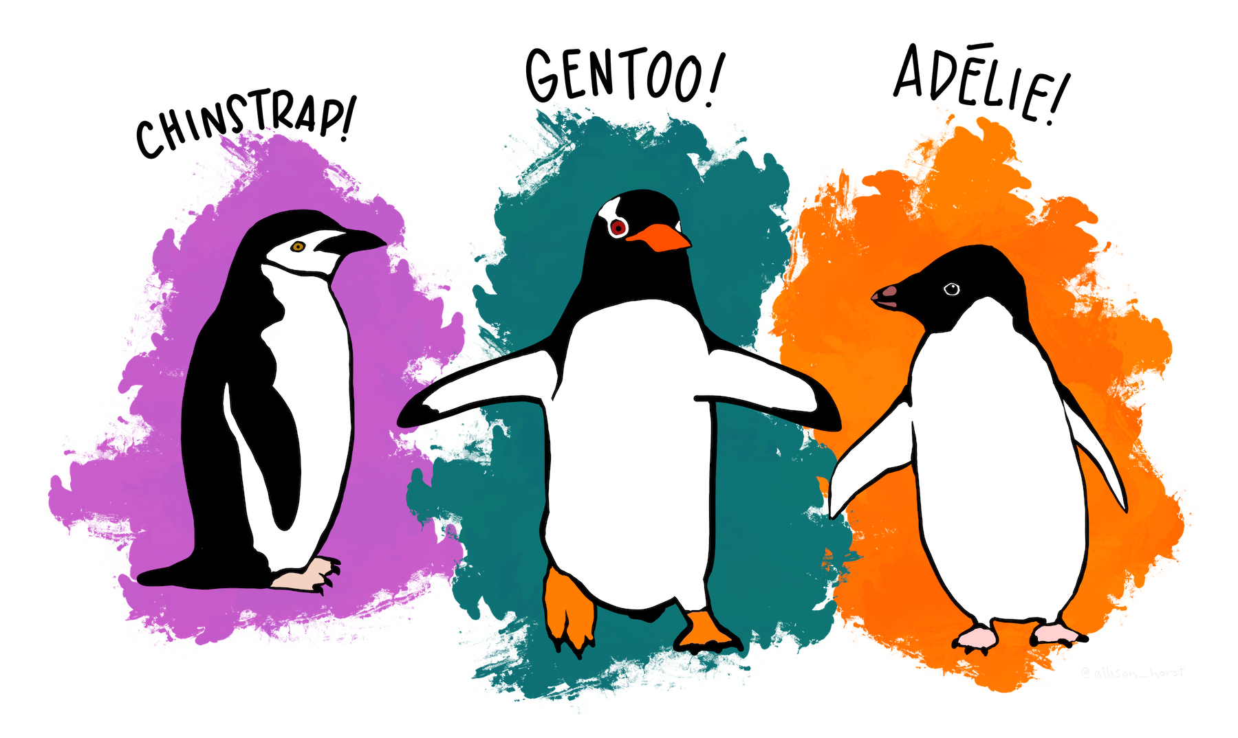
We will use penguin body mass across three species as our worked example.

⬇️ Download the companion R script: 11_anova.R

Packages needed

library(tidyverse)
library(palmerpenguins)
library(skimr)
library(car)          # Anova() Type III, leveneTest()
library(emmeans)      # pairwise contrasts post-ANOVA
library(multcompView) # compact letter display
library(broom)        # tidy() — clean model output

source("themes/r_themes_for_3_sizes.R")

The data

penguins_anova <- penguins |> drop_na(body_mass_g, species)
penguins_anova |> count(species)

Three species, 342 penguins total: Adelie (151), Chinstrap (68), Gentoo (123).

1 · What ANOVA does

ANOVA compares variation between groups to variation within groups. If groups differ more than random scatter within groups would predict, the F-statistic gets large and the p-value gets small.

\[H_0: \mu_{Adelie} = \mu_{Chinstrap} = \mu_{Gentoo}\] \[H_A: \text{at least one species mean differs}\]

Why not just run three t-tests?

Three groups → three possible pairwise t-tests. Each test has a 5% chance of a false positive. Running three independent tests gives roughly a 14% chance of at least one false positive. ANOVA controls the error rate for the overall comparison and then directs you to post-hoc tests for the pairwise follow-up.

A significant ANOVA does NOT tell you which groups differ

The F-test only tells you that at least one mean is different. You need a post-hoc test (we use emmeans) to find out which pairs differ.

2 · Descriptive statistics first

# Quick skim grouped by species
penguins_anova |> group_by(species) |> skim()

# Manual summary
stats_df <- penguins_anova |>
  group_by(species) |>
  summarise(
    n      = sum(!is.na(body_mass_g)),
    mean   = round(mean(body_mass_g,   na.rm = TRUE), 1),
    sd     = round(sd(body_mass_g,     na.rm = TRUE), 1),
    se     = round(sd(body_mass_g,     na.rm = TRUE) /
                     sqrt(sum(!is.na(body_mass_g))), 1),
    .groups = "drop"
  )
stats_df

Use sum(!is.na()) not n() for sample size

n() counts all rows including missing values. sum(!is.na(body_mass_g)) counts only the rows that have a real measurement — the correct denominator for SE and any other formula using n.

3 · Look at the data first

Always plot before running any test. Here you can already see that Gentoo penguins are larger and that there is real overlap between Adelie and Chinstrap.

Adelie, Chinstrap, and Gentoo penguins. Art by Allison Horst.

Boxplot with raw points

penguins_anova |>
  ggplot(aes(x = species, y = body_mass_g, fill = species)) +
  geom_boxplot(alpha = 0.6, outlier.shape = NA, width = 0.5) +
  geom_jitter(width = 0.15, alpha = 0.35, size = 1.5) +
  labs(x = "Species", y = "Body mass (g)",
       title = "Penguin body mass by species") +
  theme_regular() +
  theme(legend.position = "none")

Mean ± SE

penguins_anova |>
  ggplot(aes(x = species, y = body_mass_g, color = species)) +
  geom_jitter(width = 0.15, alpha = 0.3, size = 1.5) +
  stat_summary(fun.data = mean_se, geom = "pointrange",
               size = 0.9, linewidth = 1) +
  labs(x = "Species", y = "Body mass (g)",
       title = "Mean ± 1 SE body mass by species") +
  theme_regular() +
  theme(legend.position = "none")

What to look for in the plots

Do the medians look different across species?
Are the boxes similar in height? (Roughly equal heights = similar variance → good for ANOVA)
Is there overlap between groups? (Overlap does not prevent significance — ANOVA accounts for within-group variation)

4 · Fit the model

Fit ANOVA as a linear model using lm(). This is the modern R approach — it is equivalent to aov() but gives you access to more diagnostic and post-hoc tools. Use car::Anova() with type = "III" for the ANOVA table.

penguin_model <- lm(body_mass_g ~ species, data = penguins_anova)

Anova(penguin_model, type = "III")

Reading the ANOVA table

              Sum Sq  Df  F value     Pr(>F)
(Intercept) 2.03e+09   1  5765.0   < 2e-16 ***
species     1.46e+08   2   207.3   < 2e-16 ***
Residuals   5.96e+07 339

The row you care about is species:

Sum Sq — variation explained by species differences
Df — degrees of freedom = number of groups − 1 = 3 − 1 = 2
F value — the ratio of between-group to within-group variation; larger = stronger evidence
Pr(>F) — the p-value; here far below 0.05, so we reject H₀

The Residuals row is the within-group variation — the baseline noise.

car::Anova() vs base R anova()

Always use car::Anova(model, type = "III"), not base R anova(). The base function uses Type I sums of squares, which depend on the order you list variables. Type III tests each effect while accounting for all others — it is the standard for publications and the only safe choice for unbalanced designs.

5 · Check the assumptions

ANOVA has three assumptions. Check the two you can actually test.

Assumption	How to check	What you want
Independence	Study design — not testable	Fish/birds sampled independently
Normality of residuals	Q-Q plot + Shapiro-Wilk	Points on the line; p > 0.05
Equal variances	Residuals vs Fitted plot + Levene’s test	Random scatter; p > 0.05

Check residuals, not raw data

ANOVA’s normality assumption is about the residuals (observed − predicted), not the raw data. Always extract residuals from the fitted model and check those.

Residuals vs Fitted — check equal variance

diag_df <- tibble(
  fitted    = fitted(penguin_model),
  residuals = residuals(penguin_model),
  std_resid = rstandard(penguin_model)
)

ggplot(diag_df, aes(x = fitted, y = residuals)) +
  geom_point(alpha = 0.5, color = "steelblue") +
  geom_hline(yintercept = 0, linetype = "dashed", color = "tomato") +
  geom_smooth(method = "loess", se = FALSE, color = "grey40", linewidth = 0.8) +
  labs(title = "Residuals vs Fitted",
       x = "Fitted values", y = "Residuals") +
  theme_regular()

What you want: Points scattered randomly above and below zero with similar spread at all fitted values. A fan shape (spread increases left to right) means unequal variance.

Q-Q plot — check normality of residuals

ggplot(diag_df, aes(sample = std_resid)) +
  stat_qq(alpha = 0.5, color = "steelblue") +
  stat_qq_line(color = "tomato") +
  labs(title = "Normal Q-Q plot of residuals",
       x = "Theoretical quantiles",
       y = "Standardised residuals") +
  theme_regular()

What you want: Points close to the diagonal line. Curved patterns or strong deviations at the tails indicate non-normality.

Levene’s test — equal variance

leveneTest(body_mass_g ~ species, data = penguins_anova)

Shapiro-Wilk — normality of residuals

shapiro.test(residuals(penguin_model))

Interpreting the tests

Levene’s p > 0.05 → variances are not significantly different → assumption met
Shapiro-Wilk p > 0.05 → residuals are consistent with normality → assumption met
With n > 30 per group, ANOVA is fairly robust to moderate non-normality (Central Limit Theorem). Trust the Q-Q plot over the Shapiro-Wilk p-value in larger samples.

What if assumptions are violated?

Non-normality with small n → consider a Kruskal-Wallis test (non-parametric alternative)
Unequal variances → Welch’s one-way ANOVA: oneway.test(y ~ group, data = df, var.equal = FALSE)
For ecological data with large balanced samples, ANOVA is generally robust to mild violations — use your judgment and report what you found.

6 · Post-hoc tests with `emmeans`

The F-test told us at least one species differs. emmeans tells us which ones.

Estimated marginal means

penguin_emm <- emmeans(penguin_model, ~ species)
penguin_emm

This gives the estimated mean body mass for each species with its SE and 95% CI.

All pairwise contrasts — Tukey adjustment

pairs(penguin_emm, adjust = "tukey")

Reading the emmeans pairwise output

contrast                  estimate   SE  df  t.ratio  p.value
Adelie - Chinstrap           -32   68.4 339   -0.47   0.878
Adelie - Gentoo            -1375   57.9 339  -23.74   <.0001
Chinstrap - Gentoo         -1343   74.0 339  -18.15   <.0001

estimate — difference in means between the two species (negative = first is smaller)
SE — standard error of that difference
t.ratio — the t-statistic for this pairwise comparison
p.value — Tukey-adjusted p-value (already corrected for multiple comparisons)

Here: Gentoo differs from both Adelie and Chinstrap; Adelie and Chinstrap do not differ from each other.

Compact letter display (a, b, c labels)

The compact letter display gives every group a letter. Groups sharing a letter are NOT significantly different.

penguin_cld <- cld(penguin_emm, adjust = "tukey",
                   Letters = letters, sort = FALSE)
penguin_cld

 species    emmean   SE   df lower.CL upper.CL .group
 Adelie       3701   48  339     3607     3795  a
 Chinstrap    3733   73  339     3589     3877  a
 Gentoo       5076   55  339     4968     5184   b

Adelie and Chinstrap both carry the letter a (not different from each other). Gentoo carries b (different from both).

Tukey vs Sidak vs Bonferroni

Correction	When to use
Tukey	All pairwise comparisons — the standard for ANOVA post-hoc
Sidak	Similar to Tukey; slightly less conservative
Bonferroni	A small number of pre-planned comparisons

For one-way ANOVA post-hoc, Tukey is almost always the right choice.

7 · Effect size — eta-squared (η²)

A significant p-value tells you the effect is real. η² tells you how large it is.

ss_between <- sum((fitted(penguin_model) -
                     mean(penguins_anova$body_mass_g))^2)
ss_total   <- sum((penguins_anova$body_mass_g -
                     mean(penguins_anova$body_mass_g))^2)
eta_sq     <- round(ss_between / ss_total, 3)
eta_sq

Interpreting η²

η² is the proportion of total variance explained by the group factor.

η²	Interpretation
0.01	Small effect
0.06	Medium effect
0.14	Large effect

For penguin species and body mass, η² is around 0.55 — species explains roughly 55% of the total variation in body mass. That is a very large effect.

8 · Publication figure with significance letters

cld_df <- as_tibble(penguin_cld) |>
  mutate(.group = str_trim(.group))

pub_plot <- penguins_anova |>
  ggplot(aes(x = species, y = body_mass_g, fill = species)) +
  geom_boxplot(alpha = 0.6, outlier.shape = NA, width = 0.5) +
  geom_jitter(width = 0.12, alpha = 0.3, size = 1.5) +
  geom_text(data = cld_df,
            aes(x = species, y = 6400, label = .group),
            size = 5, fontface = "bold", inherit.aes = FALSE) +
  labs(
    x       = "Species",
    y       = "Body mass (g)",
    title   = "Penguin body mass by species",
    caption = paste0("One-way ANOVA; letters indicate Tukey HSD groups",
                     " (α = 0.05); η² = ", eta_sq)
  ) +
  theme_regular() +
  theme(legend.position = "none")

pub_plot

ggsave("figures/penguin_anova.pdf",
       plot = pub_plot, width = 6, height = 5, units = "in")

Figure caption format

Figure 1. Body mass (g) of three penguin species from the Palmer Archipelago. Boxplots show median and IQR; points show individual penguins. Letters above boxes indicate Tukey HSD groupings — species sharing a letter are not significantly different (α = 0.05). Gentoo penguins were significantly heavier than both Adelie and Chinstrap penguins (one-way ANOVA: F₂,₃₃₉ = 207.3, p < 0.001, η² = 0.55); Adelie and Chinstrap did not differ.

9 · How to report the result

In-text reporting format

“Body mass differed significantly among penguin species (one-way ANOVA: F₂,₃₃₉ = 207.3, p < 0.001, η² = 0.55). Gentoo penguins (mean ± SE: 5076 ± 55 g) were significantly heavier than both Adelie (3701 ± 48 g; Tukey HSD: p < 0.001) and Chinstrap (3733 ± 73 g; p < 0.001) penguins. Adelie and Chinstrap did not differ significantly from each other (p = 0.878).”

Structure: overall test → effect size → pairwise follow-up. Never lead with p — lead with the biology and use p as support.

What was improved from the M&M version

Changes made for your other course

The original M&M ANOVA script had several things worth updating if you use it elsewhere:

n() replaced with sum(!is.na()) for correct sample sizes
Base R par(mfrow) diagnostic plots replaced with ggplot versions using extracted residuals — consistent with course style and your theme
multcompView::cld() added for compact letter display — the standard way to annotate ANOVA figures
η² now computed with a clear formula and benchmarks in a callout
broom::tidy() added so model output can be extracted cleanly for reporting
Reporting template filled with actual extracted values, not placeholder X.XX text
Welch one-way ANOVA mentioned as the fallback when Levene’s test fails

Quick reference

Task	Code
Fit ANOVA	`lm(y ~ group, data = df)`
ANOVA table (Type III)	`car::Anova(model, type = "III")`
Tidy output	`broom::tidy(Anova(model, type = "III"))`
Residuals vs Fitted	`tibble(fitted = fitted(m), resid = residuals(m))` → ggplot
Q-Q plot of residuals	`ggplot(aes(sample = rstandard(m))) + stat_qq() + stat_qq_line()`
Levene’s test	`car::leveneTest(y ~ group, data = df)`
Shapiro-Wilk on residuals	`shapiro.test(residuals(model))`
Estimated marginal means	`emmeans(model, ~ group)`
Pairwise contrasts	`pairs(emm, adjust = "tukey")`
Compact letters (a,b,c)	`cld(emm, adjust = "tukey", Letters = letters)`
Eta-squared	`SS_between / SS_total` from `fitted()` and raw y
Welch one-way (unequal var)	`oneway.test(y ~ group, data = df, var.equal = FALSE)`
Add letters to plot	`geom_text(data = cld_df, aes(x=group, y=ymax+offset, label=.group))`

End of Common Code 11 — One-Way ANOVA. Next: Common Code 12 — Correlation and regression.