Paper Calibration Curve: Predicting Leaf Area from Mass

The same analysis as regression_analysis_script.R — but as a report

Introduction

To estimate leaf surface area without a leaf-area meter, we built a calibration curve. Paper of uniform stock has a constant area-per-gram, so the mass of a paper square is a near-perfect linear predictor of its area. Once we know that relationship, we can trace a leaf onto the same paper, weigh the tracing, and convert its mass to area.

• Explanatory variable (X): paper mass (g) — easy to measure on a balance
• Response variable (Y): paper area (cm²) — what we want to predict

Methods

We weighed 118 paper squares of known area (1–567 cm²) and fit a simple linear regression, area_cm2 ~ mass_g, with lm(). We checked the four regression assumptions using base R’s diagnostic plots for a fitted model, with a Shapiro–Wilk test on the residuals as a formal companion. All work was done in R with the tidyverse; this report was written in Quarto so every number and figure below is computed directly from the data.

Results

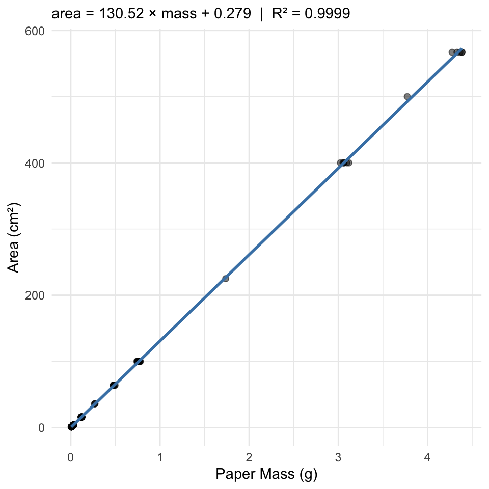
Paper mass was an extremely strong predictor of paper area. The overall model fit, coefficients, and p-values are shown in the two tables below.

Table 1. Overall fit of the calibration regression.

R-squared	F	df (model)	df (residual)	p-value
0.9999	784932.9	1	116	0

Table 2. Calibration equation coefficients. The mass_g estimate is the area gained per additional gram of paper; (Intercept) is the fitted area at zero mass.

Term	Estimate	Std. error	t	p-value
(Intercept)	0.279	0.181	1.5	0.1261386
mass_g	130.523	0.147	886.0	0.0000000

Read the calibration equation off Table 2: predicted area equals the (Intercept) estimate plus the mass_g estimate times paper mass. In words, every additional gram of paper corresponds to about the mass_g estimate in cm² of area.

Every number in Tables 1 and 2 is computed from the data when the document renders — nothing was typed by hand. Change the data file and re-render, and the tables update themselves. That is the difference from the .R script, where you would copy each number into Word yourself.

The calibration curve

Figure 1. Paper area vs. mass with the least-squares line and 95% confidence band.

Assumption checks

Figure 2. Base R diagnostic plots for the fitted model — residuals vs. fitted, normal Q-Q, scale-location, and residuals vs. leverage. A random band with no funnel or curve in panel 1 supports linearity and equal variance.

Table 3. Shapiro–Wilk normality test on the regression residuals.

W	p-value	Method
0.677	9.42496e-15	Shapiro-Wilk normality test

The Shapiro–Wilk result is in Table 3. Read W and its p-value there, then compare that verdict with the normal Q-Q panel of Figure 2.

Predicting leaf area

Table 4. Predicted leaf area for two example paper tracings, from the calibration equation.

Tracing	Mass (g)	Predicted area (cm²)
sunny-side	0.092	12.3
shady-side	0.138	18.3

Table 4 applies the calibration equation to two example tracings. The heavier shady-side tracing has the larger predicted area — consistent with our earlier finding that shady leaves are larger.

Discussion

Write one short paragraph here. Did the calibration fit well (look at R² and Figure 1)? Did the residual plot and Shapiro–Wilk support the assumptions? Why is working in area (cm²) more biologically meaningful than raw mass (g) when comparing sunny and shady leaves? This is where you paste the results paragraph you drafted in the worksheet.

References

• Whitlock, M. & Schluter, D. The Analysis of Biological Data (2nd ed.), Ch. 17.
• Wickham, H. R for Data Science (2nd ed.) — https://r4ds.hadley.nz/