Lecture: Multiple Regression

Several predictors

The multiple regression model, partial regression slopes, ANOVA and hypothesis tests for regression, assumptions and diagnostics, collinearity, interactions, dummy variables, model comparison, and predictor importance — on the Gotelli ant-diversity dataset.

Where We Left Off

Covered last time:

• Regression, t-tests, and ANOVA
• Regression assumptions
• Sum-of-squares allocation and subdivision from total sums of squares

Note

✅ Key idea from last lecture

A simple regression has one predictor and one partition of variance (regression vs. residual). Today we add more predictors — the logic barely changes, but the bookkeeping does.

Part 1 · Why Multiple Regression?

Today’s Objectives

The multiple linear regression model:

• Regression parameters
• Analysis of variance
• Null hypotheses
• Explained variance
• Assumptions and diagnostics
• Collinearity
• Interactions
• Dummy variables
• Model selection
• Importance of predictors

Note

📖 Reference

Whitlock & Schluter, Ch. 17 — Regression, and Gotelli & Ellison, A Primer of Ecological Statistics, Ch. 9 — Regression, are the core references for this lecture.

When Do We Need More Than One Predictor?

What if there’s more than one predictor (X) variable?

• If predictors are continuous
• A mix between categorical and continuous
• We can use multiple linear regression

	Continuous X	Categorical X
Continuous Y	Regression	ANOVA
Categorical Y	Logistic regression

From a Line to a (Hyper)plane

Abundance of ants can be modeled as a function of:

• latitude
• longitude
• both

Instead of a line, it’s modeled with a (hyper)plane.

What Multiple Regression Is Used For

Used in a similar way to simple linear regression:

• Describe the nature of the relationship between Y and the X’s
• Determine explained/unexplained variation in Y
• Predict new Ys from X
• Find the “best” model

The Challenges of Multiple Regression

Crawley (2012): “Multiple regression models provide some of the most profound challenges faced by the analyst”:

• Overfitting
• Parameter proliferation
• Multicollinearity
• Model selection

Stock photo of a frustrated man in a suit punching through a laptop screen, used humorously to illustrate the frustration multiple regression’s challenges (overfitting, multicollinearity, model selection) can cause.

Part 2 · The Multiple Regression Model

The Multiple Regression Model

• A set of i = 1 to n observations
• Fixed X-values for p predictor variables (X₁, X₂ … Xₚ)
• Random Y-values:

\[y_i = \beta_0 + \beta_1 x_{i1} + \beta_2 x_{i2} + ... + \beta_p x_{ip} + \epsilon_i\]

• yᵢ: value of Y for the i-th observation, X₁ = x_i1, X₂ = x_i2, …, Xₚ = x_ip
• β₀: population intercept — the mean value of Y when X₁ = 0, X₂ = 0, …, Xₚ = 0

Partial Regression Slopes

\[y_i = \beta_0 + \beta_1 x_{i1} + \beta_2 x_{i2} + ... + \beta_p x_{ip} + \epsilon_i\]

• β₁: partial regression slope — change in Y per unit change in X₁, holding other X-vars constant
• β₂: partial regression slope for X₂, holding others constant
• βₚ: partial regression slope for Xₚ, holding others constant

Note

✅ Key idea — what “partial” means

The relationship between a predictor and the response while holding all other predictors constant. It tells you the isolated effect of one variable, controlling for the influence of others.

Partial Regression Slopes — the Ant Model

Model: ant_spp ~ elevation + latitude

• The partial slope for elevation tells you how ant species richness changes with elevation when latitude is held constant
  • 1-m increase in elevation → ant spp decrease by 0.012 spp, holding latitude constant
  • Or: 100-m increase in elevation → lose 1.2 spp
• The partial slope for latitude tells you how ant species richness changes with latitude when elevation is held constant
  • 1-degree increase in latitude → ant spp decrease by 2 species, holding elevation constant
  • Moving north = fewer ant spp, even comparing sites at the same elevation

model <- lm(ant_spp ~ elevation + latitude, data = ant_df)
summary(model)

Call:
lm(formula = ant_spp ~ elevation + latitude, data = ant_df)

Residuals:
    Min      1Q  Median      3Q     Max 
-6.1180 -2.3759  0.3218  1.9070  5.8369 

Coefficients:
            Estimate Std. Error t value Pr(>|t|)   
(Intercept) 98.49651   26.50701   3.716  0.00147 **
elevation   -0.01226    0.00411  -2.983  0.00765 **
latitude    -2.00981    0.61956  -3.244  0.00427 **
---
Signif. codes:  0 '***' 0.001 '**' 0.01 '*' 0.05 '.' 0.1 ' ' 1

Residual standard error: 3.022 on 19 degrees of freedom
Multiple R-squared:  0.5543,    Adjusted R-squared:  0.5074 
F-statistic: 11.82 on 2 and 19 DF,  p-value: 0.000463

Regression Parameters — the Error Term

\[y_i = \beta_0 + \beta_1 x_{i1} + \beta_2 x_{i2} + ... + \beta_p x_{ip} + \epsilon_i\]

• εᵢ: unexplained error — the difference between yᵢ and the value predicted by the model (ŷᵢ)
• ant_spp = β₀ + β₁(lat) + β₂(elevation) + εᵢ

Tip

🖐 Notice

This is exactly the same “signal vs. noise” structure as a simple regression — just with more terms on the signal side.

Regression Parameters — Estimation

\[y_i = \beta_0 + \beta_1 x_{i1} + \beta_2 x_{i2} + ... + \beta_p x_{ip} + \epsilon_i\]

• Estimate multiple regression parameters (intercept, partial slopes) using OLS to fit the regression line
• OLS minimizes \(\sum(y_i - \hat{y}_i)^2\), the SS (vertical distance) between observed yᵢ and predicted ŷᵢ for each xᵢⱼ
• ε estimated as residuals: εᵢ = yᵢ − ŷᵢ
• Calculation solves a set of simultaneous normal equations with matrix algebra

Note

✅ Key idea

You’ll never do this matrix algebra by hand — R’s lm() does it instantly. What matters is knowing what it’s minimizing.

Regression Parameters — Prediction

The regression equation can be used for prediction by substituting new values for the predictor (X) variables.

• Confidence intervals are calculated for parameters
• Confidence and prediction intervals depend on the number of observations and predictors
  • More observations decrease interval width
  • More predictors increase interval width
• Predictions should be restricted to within the range of the X variables

Warning

⚠️ Watch out!

Extrapolating a multiple regression beyond the observed range of any predictor is riskier than in simple regression — the fitted (hyper)plane has no guarantee of being right outside the data cloud.

Part 3 · ANOVA for Multiple Regression

Partitioning Variance — Sums of Squares

Variance — \(SS_{total}\) is partitioned into \(SS_{regression}\) and \(SS_{residual}\).

• \(SS_{regression}\) is the variance in Y explained by the model
• \(SS_{residual}\) is the variance not explained by the model

Source	SS	df
Regression	\(\sum (y_i - \bar{y})^2\)	\(p\)
Residual	\(\sum (y_i - \hat{y}_i)^2\)	\(n-p-1\)
Total	\(\sum (y_i - \bar{y})^2\)	\(n-1\)

From Sums of Squares to Mean Squares

SS converted to (non-additive) MS = SS/df:

• \(MS_{residual}\): estimates population variance
• \(MS_{regression}\): estimates population variance + variation due to the strength of the X-Y relationships
• MS is an estimate of variance that doesn’t increase with sample size the way SS does

Source	SS	df	MS
Regression	\(\sum (y_i - \bar{y})^2\)	\(p\)	SS/df
Residual	\(\sum (y_i - \hat{y}_i)^2\)	\(n-p-1\)	SS/df
Total	\(\sum (y_i - \bar{y})^2\)	\(n-1\)

Hypotheses — the “Basic” Test

Two null hypotheses are usually tested in MLR. The “basic” H₀: all partial regression slopes equal 0; β₁ = β₂ = … = βₚ = 0.

• If the “basic” H₀ is true, \(MS_{regression}\) and \(MS_{residual}\) estimate the same variance, and their ratio (F-ratio) ≈ 1
• If the “basic” H₀ is false (at least one β ≠ 0), \(MS_{regression}\) estimates variance + partial regression slope effects, and the F-ratio will be > 1 — compared to the F-distribution for a p-value

Note

📖 Reference

Gotelli & Ellison, Ch. 9, covers this F-test framework for multiple regression in detail.

Hypotheses — Testing One Specific β

Also: is any specific β = 0 (explanatory role)?

• E.g., does latitude have an effect on ant species?
• These H’s are tested through model comparison
• Model 1 — with 2 predictors X₁, X₂: \(y_i = \beta_0 + \beta_1 x_{i1} + \beta_2 x_{i2} + \epsilon_i\)
• Model 2 — to test H₀ that β₂ = 0, compare the fit of Model 1 to Model 2 with 1 predictor: \(y_i = \beta_0 + \beta_1 x_{i1} + \epsilon_i\)

Tip

🖐 Notice

This is a preview of the model-comparison approach we’ll use throughout this lecture — fit two nested models and compare their fit.

Hypotheses — the Partial F-Test

• If \(SS_{regression}\) of model 1 = model 2, we cannot reject H₀: β₁ = 0 — adding X₂ did not explain any additional variance
• If \(SS_{regression}\) of model 1 > model 2, there’s evidence to reject H₀: β₂ = 0 — adding X₂ explains more variance
• SS for β₂ is \(SS_{extra,\beta_2}\) = Full \(SS_{regression}\) − Reduced \(SS_{regression}\) — this quantifies how much additional variance X₂ explains
• Use a partial F-test to test H₀: β₂ = 0:

\[F_{1,n-p} = \frac{MS_{Extra}}{Full\ MS_{Residual}}\]

Tip

🖐 Notice

R also gives you a t-test for each coefficient that answers exactly this same question — you rarely need to run the partial F-test by hand.

Explained Variance

Explained variance (r²) is calculated the same way as for simple regression:

\[r^2 = \frac{SS_{Regression}}{SS_{Total}} = 1 - \frac{SS_{Residual}}{SS_{Total}}\]

Warning

⚠️ Watch out!

• r² values cannot be used to directly compare models with different numbers of predictors
• r² values will always increase as predictors are added, even useless ones
• r² values with different transformations of Y are not comparable

Part 4 · Assumptions and Diagnostics

Assumptions and Diagnostics — Outliers

• Assume fixed X’s — unrealistic in most biological settings, but a working assumption
• No major (influential) outliers
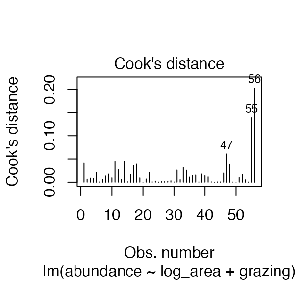
• Check leverage and influence with Cook’s Dᵢ

plot(model, which = 4)

Assumptions and Diagnostics — Residuals

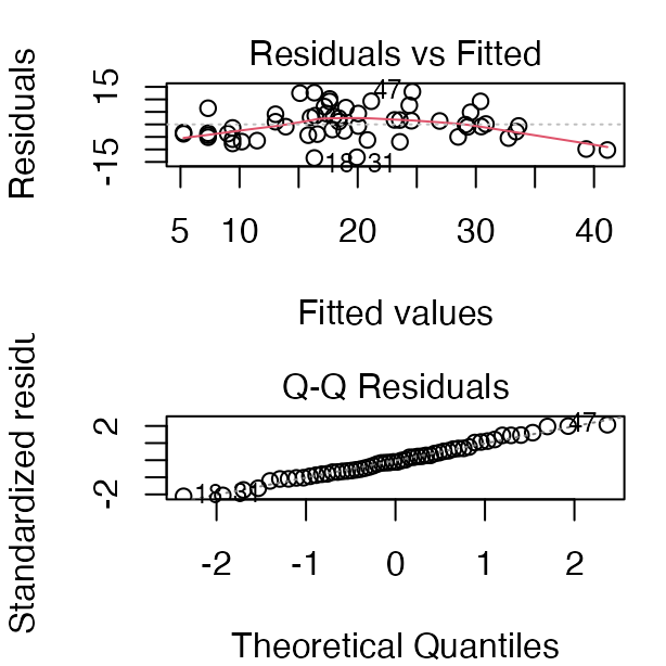
• Normality, equal variance, independence
• Residual QQ-plots, residuals-vs-predicted-values plot
• Distribution/variance issues are often corrected by transforming Y

Assumptions and Diagnostics — Sample Size and Collinearity

• More observations than predictor variables — ideally at least 10× observations than predictors, to avoid “overfitting.” 2 predictors = 20 observations, minimum!
• No collinearity — need uncorrelated predictor variables (assessed using a scatterplot matrix and VIFs)
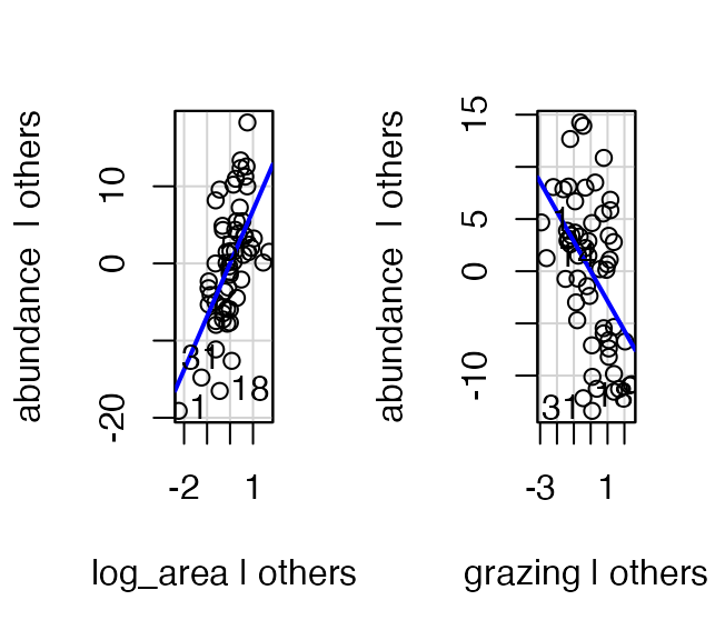
• Each X has a linear relationship with Y after accounting for other predictors — checked with Added Variable (AV) plots, also called partial regression plots

Tip

📖 AV plots in R

• All predictors: avPlots(model)
• One predictor: avPlot(model, variable = "proportion_black")

AV plots show the relationship between Y and X₁ after removing the linear effects of all other predictors.

Why Not Just Regress Y on Each X Separately?

Regressing Y vs. each X separately does not consider the effect of other predictors — but we want to know the shape of the relationship while holding other predictors constant.

Part 5 · Collinearity

Collinearity — the Problem

• Potential predictor variables are often correlated (e.g., morphometrics, nutrients, climatic parameters)
• Multicollinearity (strong correlation between predictors) causes problems for parameter estimates
• Severe collinearity causes unstable parameter estimates — a small change in a single value can result in large changes in βₚ estimates
• Inflates partial-slope error estimates, and causes a loss of power

           elevation   latitude    ant_spp
elevation  1.0000000  0.1787454 -0.5545244
latitude   0.1787454  1.0000000 -0.5879407
ant_spp   -0.5545244 -0.5879407  1.0000000

Collinearity — Detecting It

Collinearity can be detected by:

• Variance Inflation Factors (VIF): \(VIF_{X_j} = 1/(1-r^2)\); VIF > 10 = bad
• Best/simplest solution: exclude variables that are highly correlated with other variables — they’re probably measuring similar things and are redundant

Note

✅ Key idea

A high VIF doesn’t mean your model is “wrong” — it means you can’t trust the individual partial slopes for the correlated predictors, even if the overall model fits well.

Part 6 · Interactions

Interactions — Additive vs. Multiplicative

Predictors can be modeled as:

• additive (effect of temp, plus precip, plus fertility), or
• multiplicative (interactive)
• Interaction: the effect of Xᵢ depends on the level of Xⱼ
• The partial slope of Y vs. X₁ is different for different levels of X₂ (and vice versa) — measured by β₃

\[y_i = \beta_0 + \beta_1X_{i1} + \beta_2X_{i2} + \epsilon_i \quad \text{vs.} \quad y_i = \beta_0 + \beta_1X_{i1} + \beta_2X_{i2} + \beta_3X_{i1}X_{i2} + \epsilon_i\]

This leads to “curvature” of the regression (hyper)plane.

Tip

🖐 Notice

An interaction term is just another predictor: the product \(X_1 \times X_2\), fit with its own coefficient β₃.

Interactions — Curvature of the Regression Plane

Interaction terms lead to “curvature” of the regression (hyper)plane.

Interactions — the Cost

Adding interactions:

• Means many more predictors (“parameter proliferation”) — 2ⁿ terms are required; 6 parameters = 64 terms, 7 parameters = 128 terms
• Makes interpretation more complex
• When to include interactions? When they make biological sense!

Warning

⚠️ Watch out!

Don’t add interaction terms just to see if they’re significant — with enough predictors, some interaction will hit p < 0.05 by chance alone.

Part 7 · Dummy Variables

Dummy Variables

Multiple linear regression accommodates continuous and categorical variables (gender, vegetation type, etc.). Categorical vars become “dummy vars”: number of dummy variables = number of categories − 1.

• Sex M/F: need 1 dummy var with two values (0, 1)
• Fertility L/M/H: need 2 dummy vars, each with two values (0, 1): fert1 (0 if L or H, 1 if M), fert2 (1 if H, 0 if L or M)

Fertility	fert1	fert2
Low	0	0
Med	1	0
High	0	1

Dummy Variables — the Reference Condition

Coefficients are interpreted relative to a reference condition:

• R codes dummy variables automatically
• It picks the “reference” level alphabetically
• Dummy variables with more than 2 levels add extra predictor variables to the model

Fertility	fert1	fert2
Low	0	0
Med	1	0
High	0	1

Dummy Variables — Worked Example

R console output for a linear model regressing total net primary productivity on mean annual temperature, mean annual precipitation, and a three-level fertility factor (High reference, Low, Med), showing the coefficient table with all predictors highly significant (p < 0.001) and dummy-variable coefficients of 205.16 for Low and 116.33 for Medium fertility relative to High.

Boxplot of net primary productivity by fertility category (High, Low, Med), showing the Low fertility group with the highest median productivity, matching the positive dummy-variable coefficients shown in the accompanying regression output.

Part 8 · Comparing Models

Comparing Models — the Problem

When you have multiple predictors (and interactions!):

• How do you choose the “best” model?
• Which predictors should you include?
• Occam’s razor: the “best” model balances complexity with fit to the data
• To choose: compare “nested” models
• Overfitting: getting a high r² just by having more (useless) predictors — so r² alone is not a good way to choose between nested models

Note

📖 Reference

Whitlock & Schluter, Ch. 17, covers model comparison and selection for regression.

Comparing Models — Penalizing Complexity

Need to account for the increase in fit that comes just from added predictors:

• Adjusted r²
• Akaike’s Information Criterion (AIC)
• Both “penalize” models for extra predictors
• Higher adjusted r² and lower AIC are better when comparing models (p = predictors, n = sample size)

\[\text{Adjusted } r^2 = 1 - \frac{SS_{Residual}/(n - (p + 1))}{SS_{Total}/(n - 1)}\] \[\text{AIC} = n[\ln(SS_{Residual})] + 2(p + 1) - n\ln(n)\]

Comparing Models — How to Search

• Can fit all possible models, then compare AICs or adjusted r² — tedious with lots of predictors
• Automated forward (and backward) stepwise procedures: start with no terms (or all terms), add (remove) the term with the largest (smallest) partial F statistic
• We will use a manual form of backward selection

Tip

🖐 Notice

Automated stepwise selection is convenient but controversial — it can overfit and doesn’t know which predictors make biological sense. Manual, hypothesis-driven selection is usually better for a small model.

Comparing Models — the Full Model

========== FULL MODEL (Both Variables) ==========

Call:
lm(formula = ant_spp ~ elevation + latitude, data = ant_df)

Residuals:
    Min      1Q  Median      3Q     Max 
-6.1180 -2.3759  0.3218  1.9070  5.8369 

Coefficients:
            Estimate Std. Error t value Pr(>|t|)   
(Intercept) 98.49651   26.50701   3.716  0.00147 **
elevation   -0.01226    0.00411  -2.983  0.00765 **
latitude    -2.00981    0.61956  -3.244  0.00427 **
---
Signif. codes:  0 '***' 0.001 '**' 0.01 '*' 0.05 '.' 0.1 ' ' 1

Residual standard error: 3.022 on 19 degrees of freedom
Multiple R-squared:  0.5543,    Adjusted R-squared:  0.5074 
F-statistic: 11.82 on 2 and 19 DF,  p-value: 0.000463

Comparing Models — Elevation Only

========== ELEVATION ONLY MODEL ==========

Call:
lm(formula = ant_spp ~ elevation, data = ant_df)

Residuals:
    Min      1Q  Median      3Q     Max 
-4.9010 -2.6947 -0.9502  2.9657  7.6363 

Coefficients:
             Estimate Std. Error t value Pr(>|t|)    
(Intercept) 12.589088   1.385615   9.086 1.55e-08 ***
elevation   -0.014641   0.004913  -2.980   0.0074 ** 
---
Signif. codes:  0 '***' 0.001 '**' 0.01 '*' 0.05 '.' 0.1 ' ' 1

Residual standard error: 3.671 on 20 degrees of freedom
Multiple R-squared:  0.3075,    Adjusted R-squared:  0.2729 
F-statistic: 8.881 on 1 and 20 DF,  p-value: 0.0074

Comparing Models — Latitude Only

========== LATITUDE ONLY MODEL ==========

Call:
lm(formula = ant_spp ~ latitude, data = ant_df)

Residuals:
    Min      1Q  Median      3Q     Max 
-6.2223 -2.1188  0.0599  2.1267  6.4990 

Coefficients:
            Estimate Std. Error t value Pr(>|t|)   
(Intercept) 109.8532    30.9803   3.546  0.00203 **
latitude     -2.3401     0.7199  -3.251  0.00401 **
---
Signif. codes:  0 '***' 0.001 '**' 0.01 '*' 0.05 '.' 0.1 ' ' 1

Residual standard error: 3.569 on 20 degrees of freedom
Multiple R-squared:  0.3457,    Adjusted R-squared:  0.313 
F-statistic: 10.57 on 1 and 20 DF,  p-value: 0.004006

Comparing Models — Putting It Together

========== MODEL COMPARISON TABLE ==========

           Model Adjusted_R2      AIC R2_vs_Full AIC_vs_Full
1 Both Variables   0.5074180 115.8646  0.0000000    0.000000
2 Elevation Only   0.2728722 123.5608 -0.2345459    7.696164
3  Latitude Only   0.3129580 122.3132 -0.1944600    6.448613

========== KEY FINDINGS ==========

Full Model AIC: 115.86 (Adjusted R^2: 0.5074)

Elevation Only AIC: 123.56 (Adjusted R^2: 0.2729)

Latitude Only AIC: 122.31 (Adjusted R^2: 0.3130)

--- Differences from Full Model ---

Removing latitude: AIC increases by 7.70, Adj R^2 decreases by -0.2345

Removing elevation: AIC increases by 6.45, Adj R^2 decreases by -0.1945

========== CONCLUSION ==========

Full model has LOWEST AIC (best fit)

Full model has HIGHEST Adjusted R^2 (explains most variance)

Removing either variable worsens model performance

Both elevation and latitude are important predictors of ant species diversity!

Part 9 · Relative Importance of Predictors

How Important Is Each Predictor?

Usually we want to know the relative importance of predictors in explaining Y. Three general approaches:

• Using F-tests (or t-tests) on partial regression slopes
• Using the coefficient of partial determination
• Using standardized partial regression slopes

Note

✅ Key idea

None of these three approaches is “the” right answer — each answers a slightly different question about importance.

Approach 1 — F-Tests on Partial Slopes

Using F-tests (or t-tests) on partial regression slopes:

• Conduct F-tests of H₀ that each partial regression slope = 0
• If you cannot reject H₀, discard the predictor
• Can get additional clues from the relative size of F-values
• Does not tell us the absolute importance of a predictor — you usually cannot directly compare slope parameters

Warning

⚠️ Watch out!

A bigger F-value doesn’t automatically mean a “more important” predictor if the predictors are on very different scales.

Approach 2 — Coefficient of Partial Determination

The reduction in variation of Y due to adding predictor Xⱼ:

\[r_{X_j}^2 = \frac{SS_{Extra}}{Reduced\ SS_{Residual}}\]

• \(SS_{Extra}\) = increase in \(SS_{regression}\) when Xⱼ is added to the model
• Reduced \(SS_{residual}\) is the unexplained SS from the model without Xⱼ

Tip

🖐 Notice

This is the same \(SS_{Extra}\) logic from the partial F-test earlier — just expressed as a proportion of variance instead of an F-ratio.

Approach 3 — Standardized Partial Regression Slopes

Predictors on different scales cannot be directly compared — why?

• Standardize all variables (mean = 0, SD = 1)
• Scales are then identical, and a larger standardized partial slope means a more important variable

Note

✅ Key idea

Standardizing puts every predictor in “SD units,” so a slope of 0.5 always means “half an SD change in Y per SD change in X” — directly comparable across predictors.

Partial Eta Squared and Delta R²

Using partial r² values — partial eta squared (pEta²):

• Elevation: 0.3189 (31.9%) — elevation explains 31.9% of the variance after controlling for latitude
• Latitude: 0.3564 (35.6%) — latitude explains 35.6% of the variance after controlling for elevation
• Both are important predictors! Latitude is slightly stronger

Delta R² (semi-partial R²):

• Elevation: 0.2087 — if you removed elevation, R² would drop by 20.9%
• Latitude: 0.2468 — if you removed latitude, R² would drop by 24.7%
• Shows the unique contribution of each predictor to the total variance explained

== Type II ANOVA (car package) ==

Anova Table (Type II tests)

Response: ant_spp
           Sum Sq Df F value   Pr(>F)   
elevation  81.224  1  8.8955 0.007652 **
latitude   96.085  1 10.5231 0.004272 **
Residuals 173.487 19                    
---
Signif. codes:  0 '***' 0.001 '**' 0.01 '*' 0.05 '.' 0.1 ' ' 1

== Coefficients Table ==

 Coefficients    SSR df pEta_sqr dR_sqr
    elevation  81.22  1   0.3189 0.2087
     latitude  96.09  1   0.3564 0.2468
    Residuals 173.49 19   0.5000 0.4457

== Summary Statistics ==

SSE: 173.5

SST: 389.3

Model R^2: 0.5543