Lecture: Multivariate Statistics

An introduction to multivariate data, distance, and ordination

Introduction to multivariate analysis of ecological data — standardization, distance and dissimilarity metrics (Euclidean, Manhattan, Bray-Curtis, Jaccard), the dissimilarity matrix, a map of the ordination methods (PCA, PCoA, CA, NMDS, cluster analysis), first looks at PCA and NMDS, and testing group differences, using Darlingtonia (cobra lily) morphology and Doubs River fish data.

Part 1 · Why Multivariate Data?

Where We Have Been

One response variable at a time

• Everything from t-tests through ANCOVA and mixed models shared one structure:
  • One response variable, y
  • One or more predictors
  • Partition the variance in y
• That works when the biology really is about one number — lifespan, mass, count, survival.

But ecology is rarely one number

• A plant is its whole shape: height and mouth and tube and wing and mass.
• A stream site is its whole fish community: 27 species at once.
• Running 10 separate ANOVAs on 10 traits:
  • inflates the family-wise error rate,
  • and still never tells you how the traits go together.

Introduction to Multivariate Analysis

What multivariate methods do

• Take many correlated variables measured on the same objects and ask:
  • Which objects resemble which?
  • What are the main axes of variation?
  • Do groups differ in their overall multivariate makeup?
• Three jobs, in order, and this lecture is a map of all three:
  1. Put variables on a common footing — standardization
  2. Turn objects into resemblances — distance / dissimilarity
  3. Draw the resemblances in 2-D — ordination

Note

Gotelli & Ellison, A Primer of Ecological Statistics, Ch. 12 — The Analysis of Multivariate Data — is the core reference for this lecture.

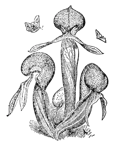
Darlingtonia californica (cobra lily)

Photo of a cobra lily (Darlingtonia californica) showing its hooded, pitcher-shaped leaves and forked, tongue-like appendages, the carnivorous plant whose morphology this lecture’s PCA example analyzes.

Our First Dataset: Darlingtonia

Cobra lily morphology

• 87 plants from 4 sites in the Siskiyou Mountains of Oregon, 10 variables each.
• Morphology (mm): height, mouth_diam, tube_diam, keel_diam, wing1_length, wing2_length, wingsprea
• Biomass (g): hoodmass_g, tubemass_g, wingmass_g
• Sites: TJH (T.J. Howell’s Fen) · DG (Day’s Gulch) · LEH (L.E. Hunter’s Fen) · HD (High Divide)

## # A tibble: 4 × 2
##   site  n_plants
##   <chr>    <int>
## 1 DG          25
## 2 HD          12
## 3 LEH         25
## 4 TJH         25

Pitcher structure showing the measured features

Vintage-style line illustration of three Darlingtonia pitcher-leaf structures with their hooded tops, tube bodies, and forked wing appendages labeled by shape, showing the plant parts behind variables like height, mouth diameter, tube diameter, and wing length/spread used in the PCA.

• All continuous, all positive, mostly correlated — the classic setting for PCA.

Our Second Dataset: Doubs River Fish

A very different kind of multivariate data

• 29 sites along the Doubs River (France), 27 fish species, abundance counts.
• Sites are ordered upstream → downstream, so there is a real environmental gradient to recover.
• The structural difference that matters:
  • 52.1% of the entries are zeros.
  • Species richness ranges from 1 to 26 species per site.
• Count data, shared absences, wildly different totals. This is why Euclidean distance is not always the right answer.

## # A tibble: 6 × 7
##    site   CHA   TRU   VAI   LOC   GAR   ABL
##   <dbl> <dbl> <dbl> <dbl> <dbl> <dbl> <dbl>
## 1     1     0     3     0     0     0     0
## 2     2     0     5     4     3     0     0
## 3    14     3     4     4     5     0     0
## 4    15     2     3     3     5     1     0
## 5    28     0     1     1     1     5     5
## 6    29     0     0     0     0     5     5

• Site 1 holds a single species (3 brown trout).
• Site 29 holds 26.
• Nothing in a t-test or an ANOVA handles a response like this.

📥 Download the Data

📥 darlingtonia.csv 📥 DoubsSpe.csv 📥 DoubsEnv.csv

Loading both datasets

darlingtonia <- read_csv("data/darlingtonia.csv")

doubs_spe <- read_csv("data/DoubsSpe.csv") %>% rename(site = 1)
doubs_env <- read_csv("data/DoubsEnv.csv") %>% rename(site = 1)

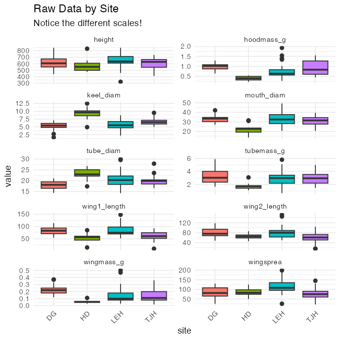
Exploring the Raw Darlingtonia Data

Always look first

• Check for outliers, examine distributions, look for patterns by site, understand the scales.
• Key observations:
  • Variables measured in different units (mm vs. g)
  • Height is in the hundreds; wing mass is in hundredths
  • We will have to standardize before we can combine them

Part 2 · Standardization

The Problem of Different Scales

Why standardization matters

• Variables with larger numbers dominate any distance you compute.
• In this data:

## # A tibble: 1 × 3
##   sd_height sd_wingmass ratio
##       <dbl>       <dbl> <dbl>
## 1      101.       0.102  986.

• Height varies about 990× more than wing mass does. In a raw Euclidean distance, wing mass contributes essentially nothing.
• That is an accident of units, not biology.

Z-score standardization

• \(Z = \dfrac{Y_i - \bar{Y}}{s}\)
• Each variable becomes:
  • Mean = 0
  • Standard deviation = 1
  • Units = “standard deviations from the mean”
• Every variable now gets an equal vote.

darl_numeric <- darlingtonia %>%
  dplyr::select(-site)

darl_scaled <- scale(darl_numeric)

Standardization in Pictures

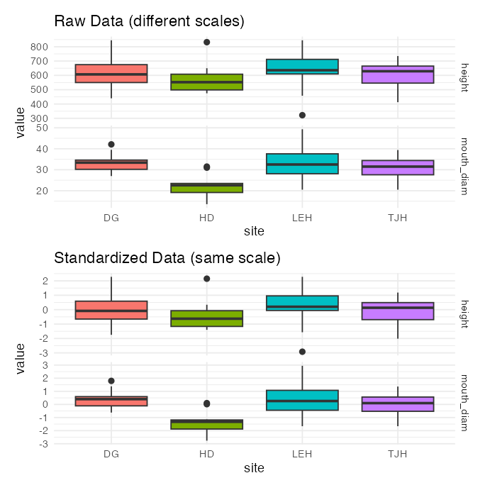
When not to standardize

• Same units, and the differences in spread are real biology.
  • Ten lengths all in mm, where “this trait varies more” is the finding — standardizing would erase it.
• Species abundance data. Standardizing each species to mean 0 turns absences into negative numbers, and most dissimilarity measures for community data are undefined for negatives.
  • Community data gets transformed (square-root, Hellinger) rather than z-scored. More on that in week 15.
• The question to ask is always: do I want these variables to have equal influence?

Part 3 · Distance and Dissimilarity

Euclidean Distance Between Two Objects

How different are two plants?

• Two variables (height, mouth diameter):
  • \(d_{i,j} = \sqrt{(y_{i,1} - y_{j,1})^2 + (y_{i,2} - y_{j,2})^2}\)
• p variables:
  • \(d_{i,j} = \sqrt{\sum_{k=1}^{p}(y_{i,k} - y_{j,k})^2}\)
• The Pythagorean theorem, extended to as many dimensions as you have variables.
• Always compute it on standardized values — otherwise you are measuring your unit choices, not your plants.

# distance between plants 1 and 2
# on the STANDARDIZED data
z <- scale(darl_numeric)

round(sqrt(sum((z[1, ] - z[2, ])^2)), 2)
## [1] 5.79

# same thing, via dist()
round(as.matrix(dist(z))[1, 2], 2)
## [1] 5.79

• 5.79 standard deviations apart across all 10 traits.

The Dissimilarity Matrix

The hub of everything that follows

• dist() returns one number for every pair of objects: an n × n dissimilarity matrix.
• With 87 plants that is 3,741 pairwise distances.
• Why it matters: PCoA, NMDS, cluster analysis, PERMANOVA and ANOSIM all start from this matrix and nothing else.
  • Choose the metric well and everything downstream is sensible.
  • Choose it badly and no amount of clever plotting rescues you.

d_darl <- dist(z)          # Euclidean

# the corner of the matrix
round(as.matrix(d_darl)[1:5, 1:5], 2)
##      1    2    3    4    5
## 1 0.00 5.79 3.50 2.36 3.73
## 2 5.79 0.00 3.27 4.74 3.78
## 3 3.50 3.27 0.00 2.40 2.03
## 4 2.36 4.74 2.40 0.00 3.45
## 5 3.73 3.78 2.03 3.45 0.00

• Symmetric, zero on the diagonal, and that is all an ordination method ever sees.

Not All Distances Are Euclidean

Four metrics you will meet in this course

Metric	Formula idea	Data it suits	Range
Euclidean	straight-line distance	continuous, standardized, few zeros	0 → ∞
Manhattan	sum of absolute differences	continuous, less outlier-sensitive	0 → ∞
Bray–Curtis	shared abundance / total abundance	species abundance counts	0 → 1
Jaccard	shared species / total species	presence–absence	0 → 1

• Euclidean and Manhattan are metric distances — they obey the triangle inequality and can be drawn in a real coordinate space.
• Bray–Curtis and Jaccard are semi-metric dissimilarities — bounded at 1 (= “share nothing”), which is exactly what you want for communities, but which breaks the geometry PCA relies on.

The Double-Zero Problem

Why community data needs Bray–Curtis

• Doubs site 1 holds one species. Site 29 holds 26. They share nothing.
• Euclidean distance counts all the species that are absent from both sites as evidence of similarity — two barren sites look like twins.
• Ecologically that is nonsense: a species can be absent for a dozen unrelated reasons.
• Bray–Curtis ignores double zeros entirely and returns 1 for two sites with nothing in common.

# sites 1 and 29 share no species
e <- as.matrix(vegdist(doubs_mat,
                       method = "euclidean"))
b <- as.matrix(vegdist(doubs_mat,
                       method = "bray"))

c(euclidean = round(e[1, 29], 2),
  bray      = round(b[1, 29], 3))
## euclidean      bray 
##      20.4       1.0

• Bray–Curtis says 1.0 — maximally different, which is correct.
• Euclidean returns a number with no upper bound and no interpretation.

Choosing a Distance Metric

Decision rules

• Continuous traits, environmental variables, few zeros
  • → standardize, then Euclidean
  • → PCA is available to you
• Species abundances with many zeros
  • → transform, then Bray–Curtis
  • → PCA is not appropriate; use NMDS or PCoA
• Presence–absence
  • → Jaccard (or Sørensen)
• Outlier-heavy continuous data
  • → Manhattan, which does not square the differences

# same data, three metrics, first pair
round(c(
  euclidean = vegdist(doubs_mat,
                 method = "euclidean")[1],
  manhattan = vegdist(doubs_mat,
                 method = "manhattan")[1],
  bray      = vegdist(doubs_mat,
                 method = "bray")[1],
  jaccard   = vegdist(doubs_mat > 0,
                 method = "jaccard")[1]), 3)
## euclidean manhattan      bray   jaccard 
##     5.385     9.000     0.600     0.667

Important

The metric is a modelling decision, not a default. It encodes what you mean by “different”.

Part 4 · Ordination — The Big Picture

What Ordination Does

Many dimensions → a readable map

• You have 10 variables, so each plant is a point in 10-dimensional space. Nobody can see that.
• Ordination finds a 2-D (or 3-D) map in which objects that were close in the full space are still close on the page.
• It is a lossy summary. Some information is always thrown away; the honest report always says how much.
• The word means “putting in order” — arranging objects along axes.

Scatterplot of a correlated two-variable Gaussian point cloud with two perpendicular black arrows overlaid, the longer arrow pointing along the direction of greatest spread (the first principal axis) and the shorter arrow perpendicular to it (the second), illustrating how PCA finds new axes aligned with the directions of maximum variance.

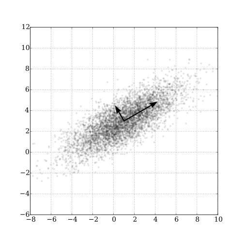
Reducing 2 variables to 1 principal axis: the new axis points along the direction of greatest spread.

The Map of Ordination Methods

Method	Starts from	Distance implied	How it solves	Where in this course
PCA	raw / standardized variables	Euclidean only	eigen-decomposition	Week 14
PCoA	any dissimilarity matrix	whatever you chose	eigen-decomposition	named only
CA / DCA	species count table	chi-square	eigen-decomposition	named only
NMDS	any dissimilarity matrix	whatever you chose	iterative, rank-based	Week 15
Cluster	any dissimilarity matrix	whatever you chose	agglomerative joining	Week 15

• The top block is eigenanalysis: one exact answer, axes ranked by variance explained, and you can read loadings off them.
• NMDS is different: it preserves only the rank order of the dissimilarities, solves by iteration, and has no “% variance explained” — it has stress instead.
• Cluster analysis answers a different question entirely: not “where does each object sit?” but “which objects group together?”

Eigenanalysis vs. Iteration

Eigen methods (PCA, PCoA, CA)

• Find axes by decomposing the correlation or distance structure directly.
• Give you:
  • an exact, reproducible answer
  • axes ordered by variance explained
  • loadings: how each variable builds each axis
• But they assume the distance is Euclidean-like and the relationships are linear.

NMDS

• Does not decompose anything. It searches: shuffle the points, measure how badly the map distorts the rank order of distances, repeat.
• Gives you:
  • a map honouring any dissimilarity you like
  • no linearity assumption
  • stress as the goodness-of-fit
• But: no loadings, axes are arbitrary, and a different random start can give a rotated answer.

Part 5 · A First Ordination — PCA

PCA in One Slide

The idea

• PCA builds new variables (components) that are:
  • Linear combinations of the original variables
  • Uncorrelated with each other
  • Ordered by how much variance they capture
• For plant i on component k:
  • \(Z_{ik} = a_{k1}Y_{i1} + a_{k2}Y_{i2} + \ldots + a_{kp}Y_{ip}\)
  • \(a_{kj}\) = the loading of variable j on component k
  • \(Z_{ik}\) = the score of plant i on component k
• PC1 takes as much variance as any single axis can; PC2 takes as much of what is left as possible, at right angles to PC1; and so on.

Running it

pca_result <- prcomp(darl_numeric,
                     center = TRUE,
                     scale. = TRUE)

• center = TRUE → mean 0
• scale. = TRUE → SD 1 (note the dot)
• Together those two arguments are the standardization from Part 2.

Note

Next week we open the box: eigenvalues, eigenvectors, and what prcomp() is actually solving.

Do the Variables Even Correlate?

PCA only helps if they do

• PCA earns its keep by collapsing redundancy. If the variables are already uncorrelated, there is no redundancy to collapse and the components are just the original variables, reordered.
• Here the strongest pairs are:

## # A tibble: 4 × 2
##   pair                            r
##   <chr>                       <dbl>
## 1 height ~ tubemass_g         0.843
## 2 wing1_length ~ wing2_length 0.836
## 3 hoodmass_g ~ wingmass_g     0.803
## 4 wing1_length ~ wingmass_g   0.764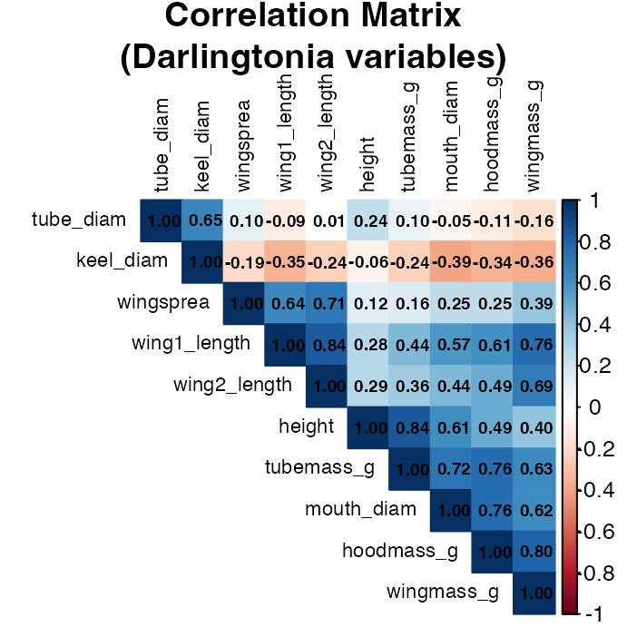

How Much Did We Capture?

Variance explained

## # A tibble: 6 × 4
##   PC    Eigenvalue Percent Cumulative
##   <chr>      <dbl>   <dbl>      <dbl>
## 1 PC1        4.99     49.9       49.9
## 2 PC2        1.77     17.7       67.5
## 3 PC3        1.53     15.3       82.8
## 4 PC4        0.573     5.7       88.5
## 5 PC5        0.352     3.5       92  
## 6 PC6        0.261     2.6       94.6

• PC1 = 49.9%, PC2 = 17.7%, PC3 = 15.3%
• First three together: 82.8% of all variation in 10 variables, in 3 numbers.

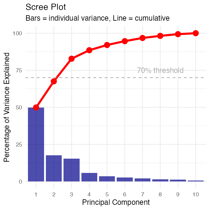
• The elbow after PC3 is the usual cue to stop.

Reading the Loadings

What loads where

##                 PC1    PC2    PC3
## height       -0.278 -0.449  0.198
## mouth_diam   -0.369 -0.110  0.214
## tube_diam     0.040 -0.602 -0.390
## keel_diam     0.202 -0.491 -0.328
## wing1_length -0.375  0.171 -0.280
## wing2_length -0.342  0.131 -0.415
## wingsprea    -0.239  0.156 -0.549
## hoodmass_g   -0.385 -0.057  0.185
## tubemass_g   -0.355 -0.320  0.263
## wingmass_g   -0.393  0.080 -0.007

Rules of thumb

• Loadings beyond ±0.3 are worth discussing; beyond ±0.5 they dominate the axis.
• Near zero means the variable has nothing to say about that axis.
• PC1: nearly every variable loads in the same direction with similar magnitude → a general size axis.
• PC2: tube_diam and keel_diam stand apart from the rest → tube girth.
• PC3: wingsprea and wing2_length dominate → a wing axis.

⚠️ The Sign of a Component Is Arbitrary

This trips up every student once

• On this run, every PC1 loading is negative. Run the same code on a different machine, or drop one plant, and they may all come back positive.
• Both answers are equally correct. An eigenvector defines a line, and a line has no preferred end. Multiplying a whole component — loadings and scores — by −1 changes nothing:
  • the variance explained is identical
  • the distances between points are identical
  • the biology is identical
• What you must never do is flip the loadings and not the scores.

# PC1 loadings are all negative here,
# so a HIGH PC1 score = a SMALL plant
round(pca_result$rotation[1:4, 1], 3)
##     height mouth_diam  tube_diam  keel_diam 
##     -0.278     -0.369      0.040      0.202

# flipping is legal and changes nothing
flip <- -pca_result$x[, 1]
round(c(var_original = var(pca_result$x[, 1]),
        var_flipped  = var(flip)), 3)
## var_original  var_flipped 
##        4.987        4.987

Always check the sign before you write a sentence such as “site X has higher PC1”. Say what it means biologically, not just which way the number went.

PC1: A Size Axis

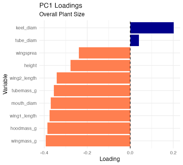
Interpretation

• Eight of ten variables load together between about −0.24 and −0.39: height, mouth, both wings, wing spread, and all three masses.
• Only keel_diam (0.202) and tube_diam (0.04) sit apart.
• Biological meaning: bigger plants are bigger in nearly every way. PC1 is general size.
• Because the loadings are negative on this run:
  • low PC1 score → large plant
  • high PC1 score → small plant

PC2 and PC3: Shape Axes

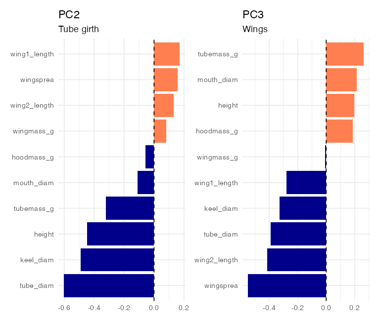
What these axes are

• PC2 (17.7%) — tube girth. tube_diam (-0.6) and keel_diam (-0.49) dominate, with height also loading. A plant can be tall and thin-tubed, or short and fat-tubed, at any overall size.
• PC3 (15.3%) — wings. wingsprea (-0.55) and wing2_length (-0.42) dominate. How far the trap’s forked appendages spread, independent of size and tube girth.
• This is PCA doing its job: three independent descriptions of shape, out of ten entangled measurements.

Scores: Putting the Plants on the Map

What scores are

• A score is one plant’s value on one component — its coordinate in the new space.
• pca_result$x holds them, one row per plant.

## # A tibble: 6 × 5
##   plant_id site    PC1   PC2   PC3
##      <int> <chr> <dbl> <dbl> <dbl>
## 1        1 TJH   -1.92  0.08  1.53
## 2        2 TJH    3.35  1.53  0.75
## 3        3 TJH    0.92 -0.03  0.25
## 4        4 TJH   -0.98  0.24 -0.24
## 5        5 TJH    1.15 -1.02  1.54
## 6        6 TJH   -1.37 -0.61  0.85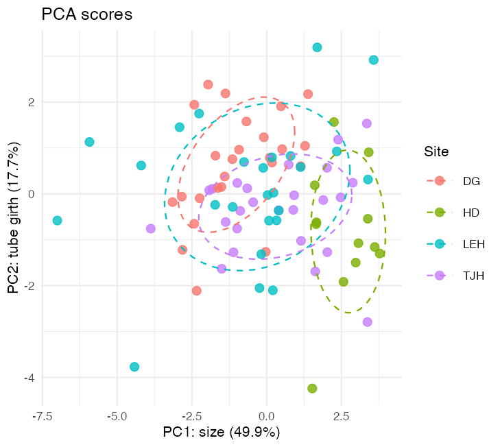

• This is an ordination: plants ordered along interpretable axes.

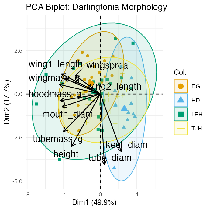
The Biplot

Reading it

• Points = plants (scores). Arrows = variables (loadings).
• Arrow length = how strongly that variable is represented in this plane.
• Angle between arrows = correlation: small angle → positively correlated; 90° → uncorrelated; 180° → negatively correlated.
• A plant lying out along an arrow is high in that variable.
• HD plants sit to the right — and because PC1 loadings are negative, right means small. HD grows the smallest plants.

Part 6 · A First NMDS

Why the Fish Data Needs a Different Tool

PCA would be the wrong choice here

• 52.1% zeros, counts spanning orders of magnitude, and a strong non-linear gradient from headwater to lowland.
• PCA would impose Euclidean distance, treat shared absences as similarity, and spread the sites along a meaningless horseshoe.
• NMDS instead:
  1. Compute Bray–Curtis dissimilarities.
  2. Drop the sites onto a 2-D map at random.
  3. Nudge them until the rank order of map distances matches the rank order of real dissimilarities as closely as possible.
  4. Report stress — how badly it still fails.

nmds <- metaMDS(doubs_mat,
                distance = "bray",
                k = 2, trymax = 50,
                trace = 0)

round(nmds$stress, 3)
## [1] 0.074

• Stress rules of thumb: < 0.05 excellent · < 0.1 good · < 0.2 usable · > 0.3 meaningless.

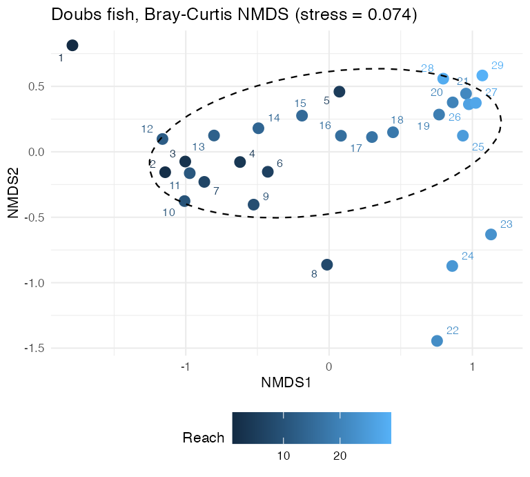
The NMDS Map

What to notice

• Sites arrange along a gradient, in roughly their real upstream-to-downstream order — which NMDS was never told.
• Stress = 0.074: a good 2-D fit.
• The axes mean nothing. No variance explained, no loadings; the map can be rotated or reflected freely.
• Contrast the PCA biplot, whose axes carried percentages and whose arrows carried meaning.

Note

Week 15 takes this apart properly: the algorithm, Shepard diagrams, choosing k, and fitting environmental vectors.

Part 7 · Testing Group Differences

Do the Sites Actually Differ?

Route 1 — ANOVA on component scores

• PC scores are ordinary continuous variables, and they are uncorrelated with one another by construction — so you may put them straight into the ANOVA you already know.
• One test per component, each answering a different question about shape.

map_dfr(c("PC1", "PC2", "PC3"), \(k) {
  a <- summary(aov(pc_scores[[k]] ~ pc_scores$site))[[1]]
  tibble(PC = k, F = round(a[1, 4], 2),
         p = signif(a[1, 5], 3))
})
## # A tibble: 3 × 3
##   PC        F          p
##   <chr> <dbl>      <dbl>
## 1 PC1    11.3 0.00000275
## 2 PC2     4.6 0.00502   
## 3 PC3    13.8 0.00000022

What it says

• All three components differ significantly among sites.
• Sites differ in size (PC1), in tube girth (PC2) and in wing spread (PC3) — the sites are not simply scaled versions of one another.
• The caveat: this is three tests on three axes chosen by the data themselves. It is a reasonable description, not a clean confirmatory test.

Warning

PCA was run on all 87 plants at once, ignoring site. The components are therefore not independent of the grouping you then test. Treat these p-values as exploratory.

Which Sites Differ, and How?

##  site emmean    SE df lower.CL upper.CL .group
##  DG   -1.024 0.383 83   -1.786   -0.262  a    
##  LEH  -0.659 0.383 83   -1.421    0.103  ab   
##  TJH   0.423 0.383 83   -0.339    1.185   b   
##  HD    2.626 0.553 83    1.526    3.726    c  
## 
## Confidence level used: 0.95 
## P value adjustment: tukey method for comparing a family of 4 estimates 
## significance level used: alpha = 0.05 
## NOTE: If two or more means share the same grouping symbol,
##       then we cannot show them to be different.
##       But we also did not show them to be the same.

Reading it in biology, not in numbers

• HD sits alone in its own group with the highest PC1 score.
• PC1 loadings are negative, so a high score means a small plant: HD grows the smallest cobra lilies, and significantly so.
• DG sits at the other end — the largest plants.
• LEH and TJH overlap in the middle.

Important

This is the sign trap in action. “HD has the highest PC1” and “HD has the smallest plants” are the same sentence. Always translate before you write.

Route 2 — PERMANOVA on the Distance Matrix

Test the whole community at once

• PERMANOVA skips the ordination entirely: it partitions the dissimilarity matrix directly and gets its p-value by permuting group labels.
• One test on all 10 variables at once, instead of one per component.

adonis2(darl_scaled ~ site,
        data   = darlingtonia,
        method = "euclidean")
## Permutation test for adonis under reduced model
## Permutation: free
## Number of permutations: 999
## 
## adonis2(formula = darl_scaled ~ site, data = darlingtonia, method = "euclidean")
##          Df SumOfSqs      R2      F Pr(>F)    
## Model     3    213.7 0.24849 9.1483  0.001 ***
## Residual 83    646.3 0.75151                  
## Total    86    860.0 1.00000                  
## ---
## Signif. codes:  0 '***' 0.001 '**' 0.01 '*' 0.05 '.' 0.1 ' ' 1

Why it is worth knowing now

• No normality assumption, no multivariate normality, no equal covariance matrices.
• Works on any dissimilarity you can justify — which is why it is the natural partner to NMDS.
• R2 is the fraction of total dissimilarity attributable to site — read it like an ANOVA’s \(\eta^2\).

PERMANOVA’s One Real Assumption

Equal dispersion

• A significant PERMANOVA means groups differ in centroid (location) or merely in spread (dispersion).
• betadisper() tells them apart.

disp <- betadisper(
  vegdist(darl_scaled, method = "euclidean"),
  darlingtonia$site)

anova(disp)
## Analysis of Variance Table
## 
## Response: Distances
##           Df  Sum Sq Mean Sq F value  Pr(>F)  
## Groups     3  11.629  3.8762   2.743 0.04828 *
## Residuals 83 117.290  1.4131                  
## ---
## Signif. codes:  0 '***' 0.001 '**' 0.01 '*' 0.05 '.' 0.1 ' ' 1

Reading the two together

• Significant PERMANOVA + non-significant dispersion → groups genuinely sit in different places. Clean result.
• Both significant → the location difference may be partly a spread difference. Say so.

round(tapply(disp$distances,
             darlingtonia$site, mean), 2)
##   DG   HD  LEH  TJH 
## 2.17 1.98 2.98 2.44

• Here both are significant: LEH is the most variable. The site effect is strong enough (R² = 0.25) that it is not only dispersion — but an honest write-up mentions it.

Note

Week 15 develops PERMANOVA and ANOSIM in full on the Doubs data.

Part 8 · Choosing a Method and Wrapping Up

A Decision Guide

Your data	Your question	Use
Continuous traits, correlated, few zeros	What are the main axes of variation?	PCA (week 14)
Species counts, many zeros	How do communities arrange along a gradient?	NMDS (week 15)
Any dissimilarity matrix	Which objects group together?	Cluster analysis (week 15)
Any dissimilarity matrix	Do my groups differ?	PERMANOVA / ANOSIM (week 15)
Continuous, multivariate normal	Do groups differ, parametrically?	MANOVA
Categorical variables	Same questions, categorical data	CA / MCA

• Two questions settle almost every case:
  1. What kind of data is it? → fixes the distance metric.
  2. Description or test? → fixes ordination vs. PERMANOVA.

Assumptions and Things That Go Wrong

Check before you ordinate

• Sample size: at least 3× as many objects as variables; 50+ is comfortable. We have 87 plants and 10 variables.
• Correlation: if nothing correlates, PCA has nothing to collapse. KMO() gives a sampling-adequacy score; ours is 0.76 (> 0.6 acceptable, > 0.8 good).
• Linearity: eigen methods see only linear relationships.
• Outliers: one extreme object can define an entire component.

Common mistakes

• ❌ Not standardizing variables with different units
• ❌ Euclidean distance on species counts
• ❌ Reading meaning into a sign flip
• ❌ Interpreting components that explain 3% of the variance
• ❌ Quoting “% variance explained” for an NMDS — it has none
• ❌ Calling a significant PERMANOVA a centroid difference without checking dispersion
• ❌ Treating an exploratory ordination as a confirmatory test

Reporting Multivariate Results

Methods

“Ten morphological and biomass variables measured on 87 Darlingtonia californica plants from four sites were standardized to zero mean and unit variance and subjected to principal component analysis (prcomp(), R 4.6.2). Components with eigenvalues > 1 were retained. Site differences were tested with PERMANOVA on Euclidean distances (vegan::adonis2(), 999 permutations), with homogeneity of multivariate dispersion checked using betadisper().”

Results — always state

1. % variance for every component you interpret
2. Loadings for the retained components
3. The biological reading of each axis, sign resolved
4. The test result with its dispersion check

Never report

• All 10 components when 3 are meaningful
• Loadings below |0.3|
• Raw eigenvalues in place of percentages
• Every individual score

Summary

What we did today

• Standardized 10 variables onto a common footing, because units are not biology.
• Built a dissimilarity matrix and learned that the choice of metric — Euclidean, Manhattan, Bray–Curtis, Jaccard — is the modelling decision.
• Saw the map of ordination methods and where each one lives in this course.
• Ran a PCA: 10 variables → 82.8% of the variation in three interpretable axes (size, tube girth, wings).
• Ran an NMDS on fish counts and recovered a river gradient at stress = 0.074.

What to carry forward

• The distance matrix is the hub. Everything downstream reads from it.
• Component signs are arbitrary — translate into biology before you write a sentence.
• Ordination describes; PERMANOVA tests. Do not confuse them.
• Next week: what prcomp() is actually solving — eigenvalues, eigenvectors, and PCA in full.
• Week 15: NMDS, cluster analysis, PERMANOVA and ANOSIM in full.

Readings

• Gotelli & Ellison, A Primer of Ecological Statistics, Ch. 12 — The Analysis of Multivariate Data
• Quinn & Keough, Experimental Design and Data Analysis for Biologists, Ch. 15 (introduction to multivariate analyses) and Ch. 16 (multivariate analysis of variance and discriminant analysis)
• Whitlock & Schluter does not cover multivariate methods.

Data sources

• Darlingtonia: Ellison, A.M. & Farnsworth, E.J. — cobra lily morphology from four sites in the Siskiyou Mountains, Oregon; distributed with Gotelli & Ellison.
• Doubs River fish: Verneaux, J. (1973), as distributed in Borcard, Gillet & Legendre, Numerical Ecology with R.