Lecture: Probability & Inference

From the normal curve to the confidence interval

The normal distribution, standardizing to the standard normal, z-scores and areas under the curve, checking the normality assumption, standard error, confidence intervals, the t-distribution, and one- and two-tailed hypothesis testing — on the Arctic grayling length dataset.

Probability and Statistical Inference

Today we build one chain of reasoning, start to finish:

1. Real data have a distribution
2. Any normal distribution can be standardized to standard normal distribution
3. Area under that curve is probability
4. All of it assumes normality — so we check
5. From one fish to the mean: SD, SE, confidence intervals
6. When σ is unknown we use the t-distribution the safe alternative
7. Putting a number on evidence: hypothesis tests

📥 Download the data

Part 1 · From data to a distribution

The normal distribution

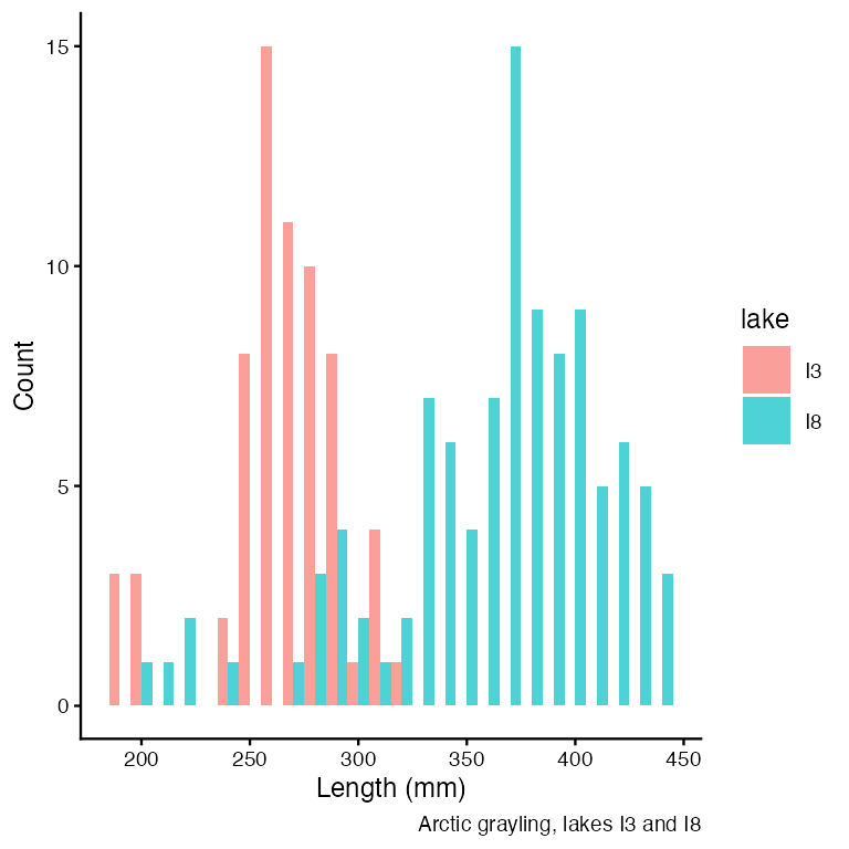
A probability distribution spreads probability across the possible outcomes — but how depends on the data:

• Discrete (a die): each outcome has its own probability, P(4) = 1/6
• Continuous (fish length): any exact value has probability zero. Probability lives in ranges, as area under the curve

The curve’s height is a density — probability per mm, not a probability. Density × width ≈ probability.

Density is a rate, so it is not capped at 1: dnorm(0, sd = 0.1) = 3.989. Nothing is 399% likely — proof that height ≠ probability.

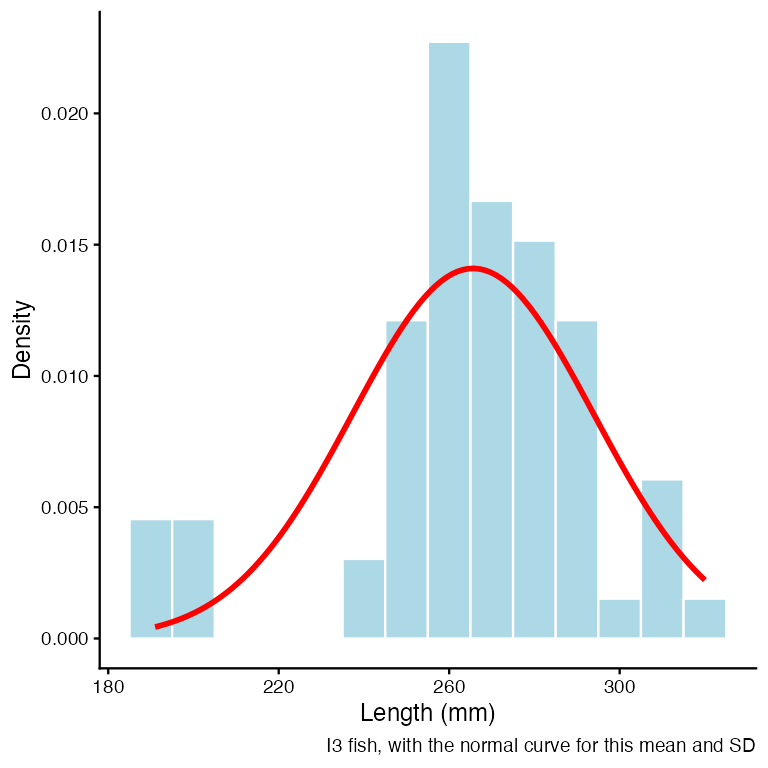
The normal is the density we lean on: symmetric, fixed by μ (where it sits) and σ (how wide), total area 1.

Lake I3: μ ≈ 265.6 mm, σ ≈ 28.3 mm — our curve. Every dataset has its own.

Note

📖 Reference

Whitlock & Schluter Ch. 10 — The Normal Distribution.
Gotelli & Ellison Ch. 2 — Random Variables and Probability Distributions.

Why we standardize

There is a different normal curve for every μ and σ. Nobody can tabulate infinitely many curves.

So we rescale every value into the same units — standard deviations from the mean:

\(z = \frac{x_i - \mu}{\sigma}\)

• \(x_i\) = the observation
• \(μ\) = mean of the distribution
• \(σ\) = standard deviation of the distribution

Subtracting μ slides the curve to centre 0. Dividing by σ squeezes it to width 1.

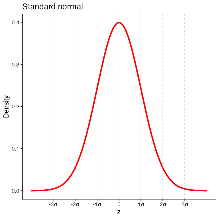
The result is the standard normal distribution: μ = 0, σ = 1. One curve. One table.

A z-score is not a new measurement. It is the same fish, expressed as “how many SDs from average.”

Practice 1 · Standardize the I3 fish

Tip

z = (length − mean) / standard deviation

i3_mean <- mean(i3_df$length_mm, na.rm = TRUE)
i3_sd   <- sd(i3_df$length_mm,   na.rm = TRUE)

i3_df <- i3_df %>%
  mutate(z_score = (length_mm - i3_mean) / i3_sd)

i3_df %>%
  select(lake, length_mm, z_score) %>%
  head(4)

# A tibble: 4 × 3
  lake  length_mm z_score
  <chr>     <dbl>   <dbl>
1 I3          266  0.0139
2 I3          290  0.862 
3 I3          262 -0.127 
4 I3          275  0.332 

A fish of 266 mm gets z = 0. A fish one SD above average gets z = 1.

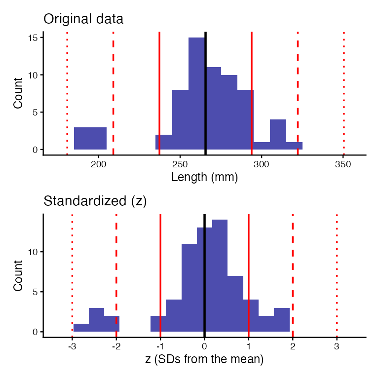
The same fish, two sets of units

Standardizing changes the axis labels, not the shape.

• Top: millimetres, centred near 266
• Bottom: z, centred at 0
• Same fish, same bars, same skew — only the ruler changed

That matters: standardizing does not make non-normal data normal. It only puts it on a common ruler. We come back to this in Part 3.

Part 2 · Area under the curve is probability

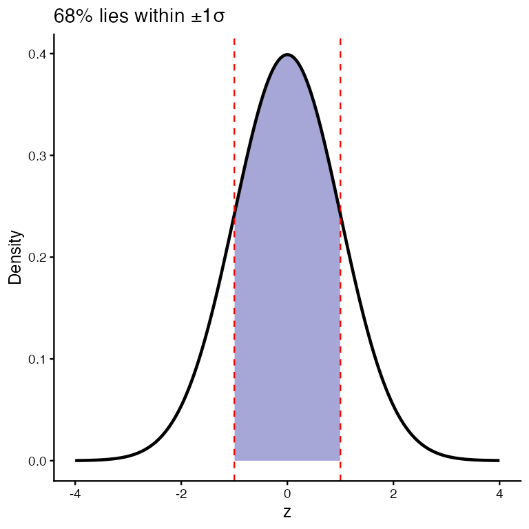
The 68–95–99.7 rule

Because the standard normal is one fixed curve, its areas are fixed too:

• 68% of the curve within ±1σ
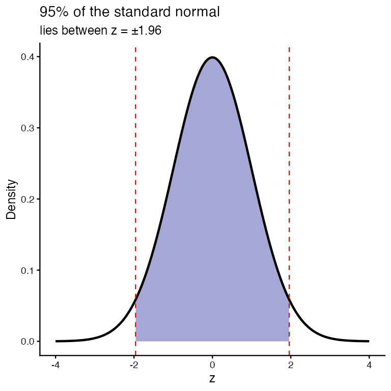
• 95% within ±1.96σ — “±2” is the rule of thumb, 1.96 is the number
• 99.7% within ±3σ

Our I3 fish, counted directly:

within_1sd <- mean(abs(i3_df$z_score) <= 1, na.rm = TRUE)
round_half_up(100 * within_1sd, 1)   # percent within 1 SD

[1] 81.8

Theory says 68%. We get 81.8%.

Hold that gap. It is the whole point of Part 3.

pnorm, qnorm, dnorm — which is which

All three describe the same standard normal curve. They differ in what you hand them and what you get back.

Function	You give it	You get back
pnorm(z)	a z	the area to the left of it
qnorm(p)	an area	the z that cuts it off
dnorm(z)	a z	the height of the curve

• p = probability, q = quantile — and they are inverses
• dnorm is the curve’s height, used to draw it. A height is not a probability — only area is

pnorm(1.96)     # area left of 1.96

[1] 0.9750021

qnorm(0.975)    # the z that puts 97.5% on its left

[1] 1.959964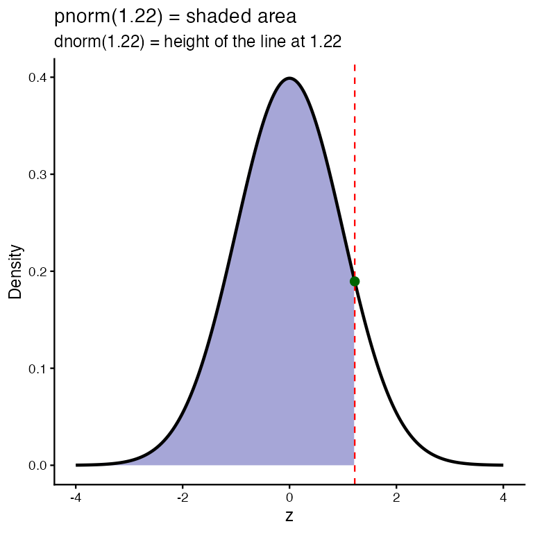

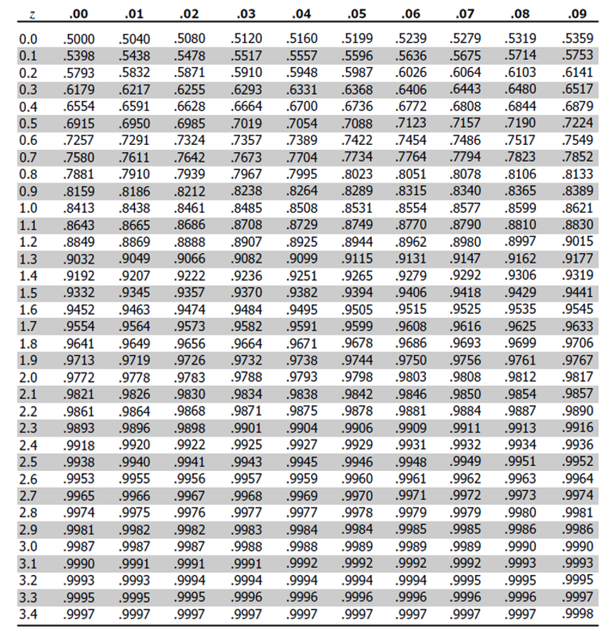
Reading the z-table

The z-table is pnorm() printed on paper: cumulative area to the LEFT of z.

• Find the ones and tenths of z down the left column
• Find the hundredths across the top
• Read the area where they meet

One table works for every dataset — because every dataset gets standardized first. (Contrast the t-table later, which needs a row for each sample size.)

Note

📖 Reference

Whitlock & Schluter Ch. 10 — standardizing a value and reading the standard normal table.

Worked example — how rare is a 300 mm grayling?

Step 1 — standardize.

\(z = \frac{300 - 265.61}{28.3} = 1.22\)

Step 2 — look it up. Row 1.2, column 0.02 → 0.8888

Step 3 — read it as biology.

• 88.9% of I3 fish are shorter than 300 mm
• 100 − 88.9 = 11.1% are longer

Catch 100 fish in I3 and about 11 should beat 300 mm.

Same answer, in R — no table:

z_fish <- (300 - i3_mean) / i3_sd
round_half_up(z_fish, 2)              # 1.22, matches the table

[1] 1.22

round_half_up(100 * (1 - pnorm(z_fish)), 1)   # % longer than 300 mm

[1] 11.2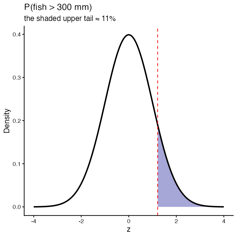

Running it backwards — qnorm

The table question can be asked the other way round, and in fisheries it usually is:

We had a length and wanted a probability. Now we have a probability and want a length.

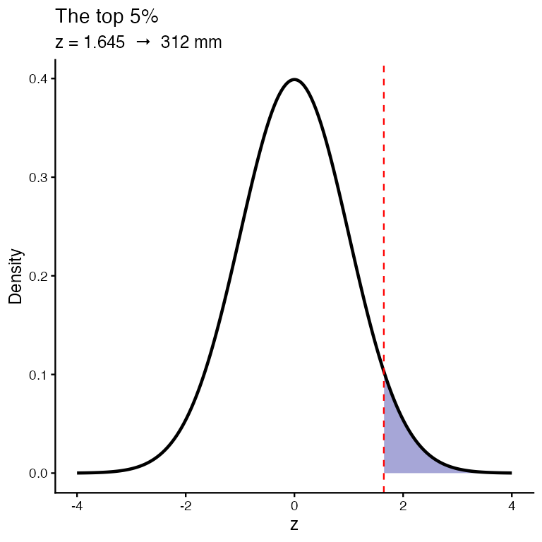
“How big must a grayling be to land in the top 5%?” — the trophy-fish question, and the size-limit question.

• qnorm(0.95) = 1.645 — the z with 5% above it
• Back to millimetres: \(x = \mu + z\sigma\)

z_top5 <- qnorm(0.95)
length_top5 <- i3_mean + z_top5 * i3_sd
round_half_up(length_top5, 1)   # mm

[1] 312.2

Only 5% of I3 fish should exceed 312.2 mm.

Every number on this slide assumed the fish are normal. Do we know that?

Part 3 · Checking the assumption

Shapiro-Wilk — and its backwards logic

The Shapiro-Wilk test asks one question, and its hypotheses run opposite to what you expect:

• H₀: the data ARE normal
• Hₐ: the data are NOT normal

So:

• p > 0.05 → no evidence against normal → carry on
• p < 0.05 → evidence of non-normality → be careful

A small p-value here is bad news, not a result. That reversal is why this test gets misread every semester.

Two cautions: with large n it flags departures too small to matter; with small n it misses ones that matter. Always read the Q-Q plot too — points on the line = normal.

shapiro.test(i3_df$length_mm)

    Shapiro-Wilk normality test

data:  i3_df$length_mm
W = 0.91051, p-value = 0.0001623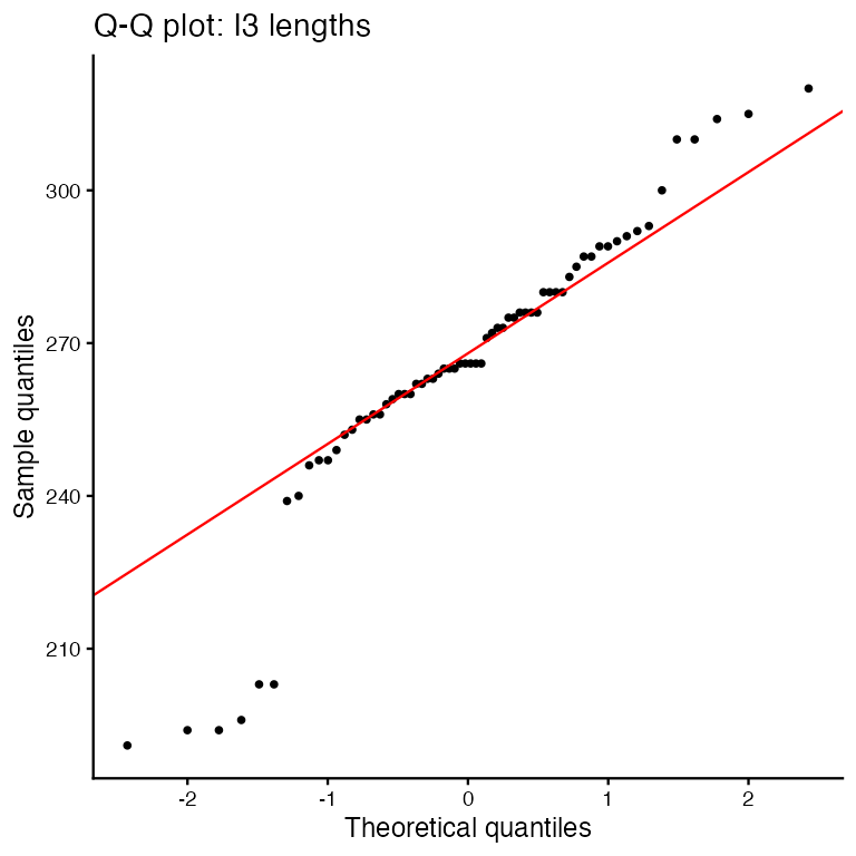

So how wrong were we?

p = 0.0002. The I3 fish are not normal. Every probability in Part 2 assumed they were — so let’s audit them against the fish themselves.

	normal theory	actual data
within ±1 SD	68%	81.8%
95th percentile	312.2 mm	310 mm
P(fish > 300 mm)	11.2%	7.6%

The centre is fine. The tail is off by a third.

And the tail is exactly where inference lives — critical values, rejection regions, p-values all sit out in the tails.

This is why we check assumptions before trusting a p-value.

Note

📖 Reference

Whitlock & Schluter Ch. 13 — Handling Violations of Assumptions.

# theory vs. the actual fish, out in the tail
round_half_up(100 * (1 - pnorm(300, i3_mean, i3_sd)), 1)

[1] 11.2

round_half_up(100 * mean(i3_df$length_mm > 300, na.rm = TRUE), 1)

[1] 7.6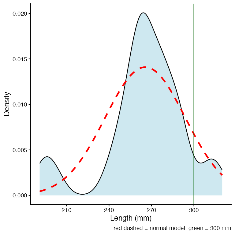

Part 4 · From one fish to the mean

SD and SE answer different questions

Everything so far described individual fish. Science usually asks about the mean. Those need different spreads.

Question	Spread
How long is a single fish?	SD (s)
Where is the population mean?	SE (s/√n)

• Fish spread is however wide the fish are — more fish does not narrow it
• Mean spread shrinks as n grows — averages are steadier than individuals
• “5% of fish exceed 312.2 mm” uses SD; “the mean is near 265.6” uses SE

Using SE where you meant SD makes your interval √n times too narrow.

i3_n  <- sum(!is.na(i3_df$length_mm))
i3_se <- i3_sd / sqrt(i3_n)

tibble(
  n  = i3_n,
  SD = round_half_up(i3_sd, 1),
  SE = round_half_up(i3_se, 1)
)

# A tibble: 1 × 3
      n    SD    SE
  <int> <dbl> <dbl>
1    66  28.3   3.5

What a confidence interval actually is

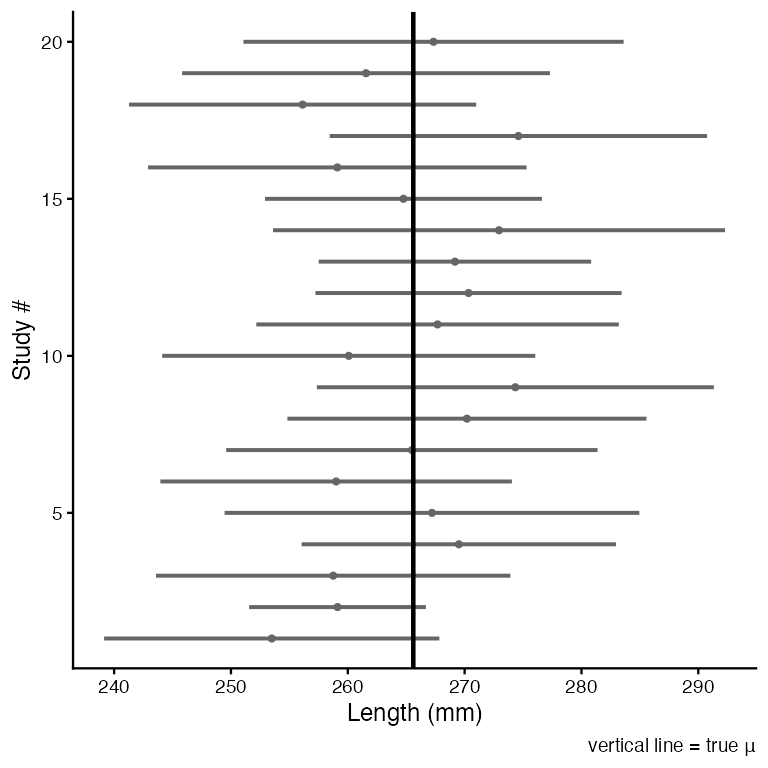
We have one sample and one mean, 265.6 mm. The true μ is some other number we will never see. A confidence interval is our honest statement of how close we probably are.

The recipe: \(\bar{y} \pm (\text{critical value}) \times SE\)

What “95%” means: repeat the whole study many times, build an interval each time, and 95% of those intervals will contain μ. The figure shows 20 such studies — one misses.

Warning

The interpretation everyone gets wrong

❌ “There is a 95% chance μ is in my interval.”

✅ “95% of intervals built this way capture μ.”

μ is a fixed number — it is not moving around. The interval is what is random. Yours either caught μ or it didn’t; you don’t get to know which.

If we knew σ, we would use z

When the population σ is genuinely known, the critical value comes straight off the standard normal:

\(CI = \bar{y} \pm 1.96 \cdot \frac{\sigma}{\sqrt{n}}\)

• 1.96 because 95% of the standard normal lies within ±1.96
• 90% CI → 1.645 · 99% CI → 2.576 · all from qnorm()

qnorm(0.975)   # 95%

[1] 1.959964

qnorm(0.95)    # 90%

[1] 1.644854

Wider confidence costs a wider interval. You cannot be more certain and more precise at the same time — only a bigger n buys you both.

But we never know σ — so z is too confident

Look again at that formula. It needs σ, the population standard deviation. We have never once had it.

What we actually have is s, computed from our 66 fish. And s is itself an estimate — a different sample gives a different s.

Two sources of uncertainty, not one:

1. the mean wobbles from sample to sample
2. our estimate of the spread also wobbles

Using 1.96 accounts for the first and ignores the second. Intervals come out too narrow and we claim more precision than we earned.

Gosset hit exactly this at Guinness — tiny barley samples, σ never known. His fix: use a curve with fatter tails, so the critical value is bigger and the interval honest.

That curve is Student’s t.

The t-distribution

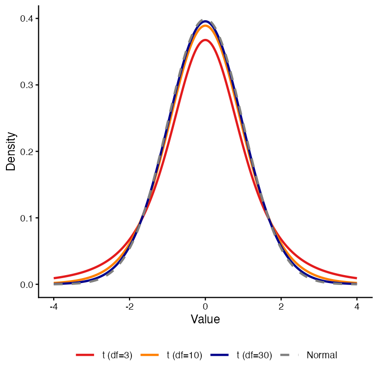
Same bell shape as the normal, but heavier in the tails — that extra thickness is the price of estimating σ.

• Shape set by degrees of freedom, df = n − 1
• Small df → very heavy tails → large critical values
• df grows → t creeps toward the normal
• Past n ≈ 30 they agree to about two decimals — which is where the “n > 30” rule of thumb came from

Important

The rule that matters: whenever σ is estimated from the sample, use t — at any sample size. “n > 30, use z” is a convenience from the era of paper tables, not a statistical law. R uses t always.

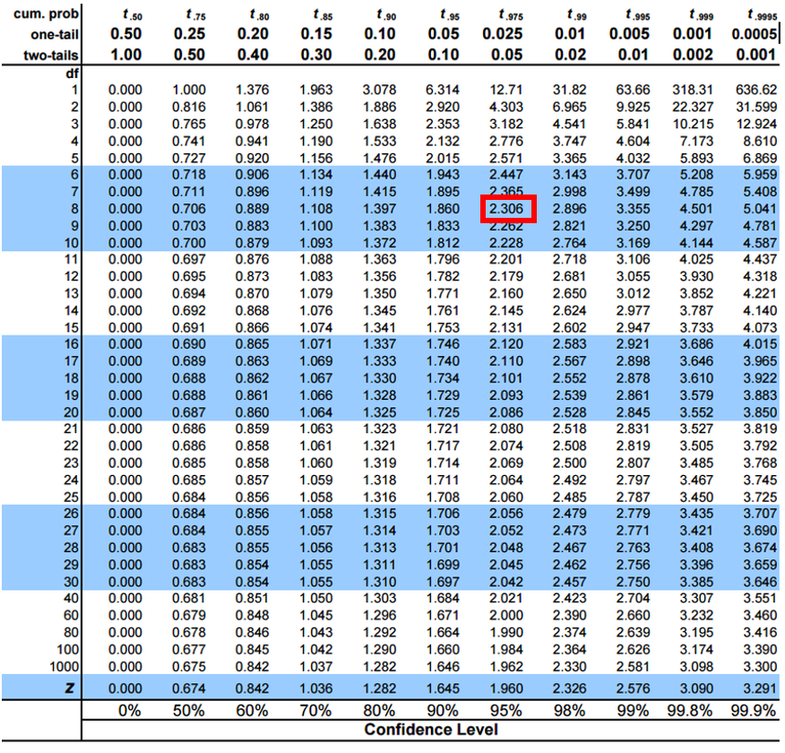
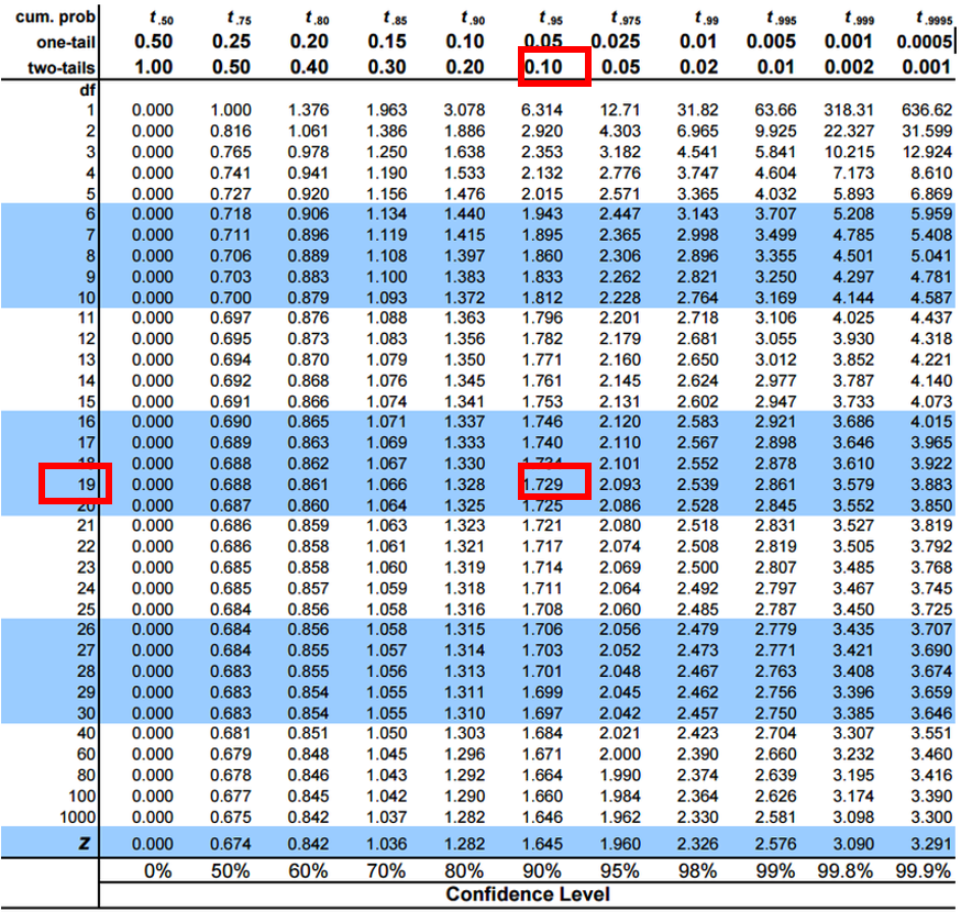
Reading the t-table

\(CI = \bar{y} \pm t \cdot \frac{s}{\sqrt{n}}\)

Only the multiplier changed: t in place of 1.96.

• Rows = degrees of freedom (n − 1)
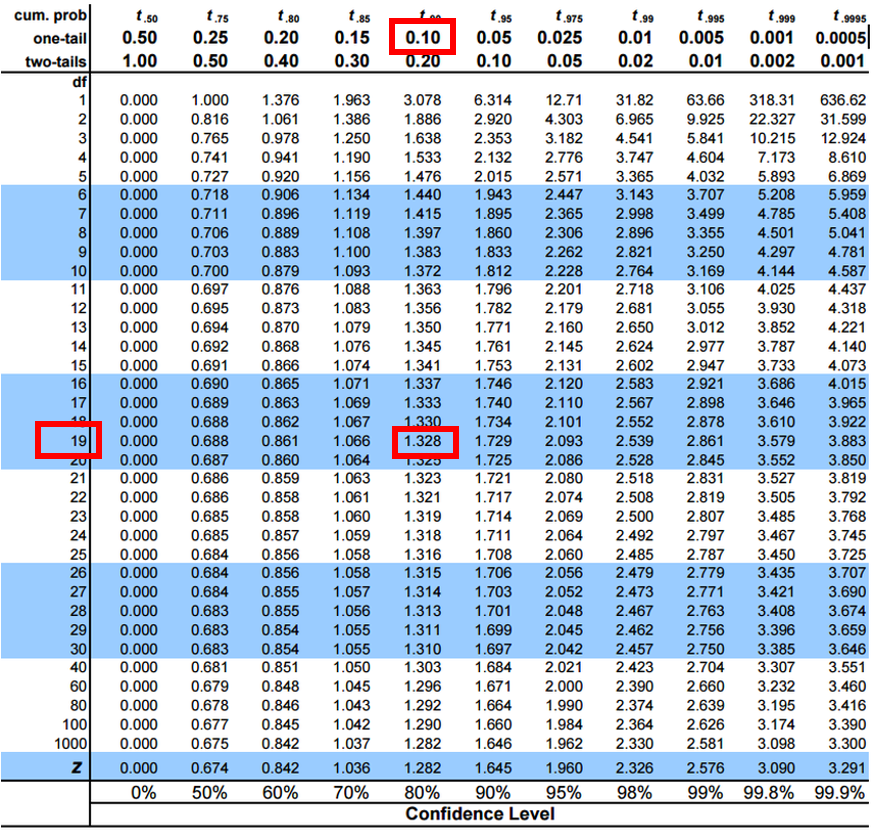
• Columns = probability, with two header rows: one-tail and two-tail
• A CI is always two-tailed — it has two ends. Use the two-tail column

The bottom row (df = ∞) is 1.96: the t-table contains the z-table.

qt(0.975, df = 8)    # 95% CI, n = 9

[1] 2.306004

qt(0.975, df = 65)   # 95% CI, n = 66

[1] 1.997138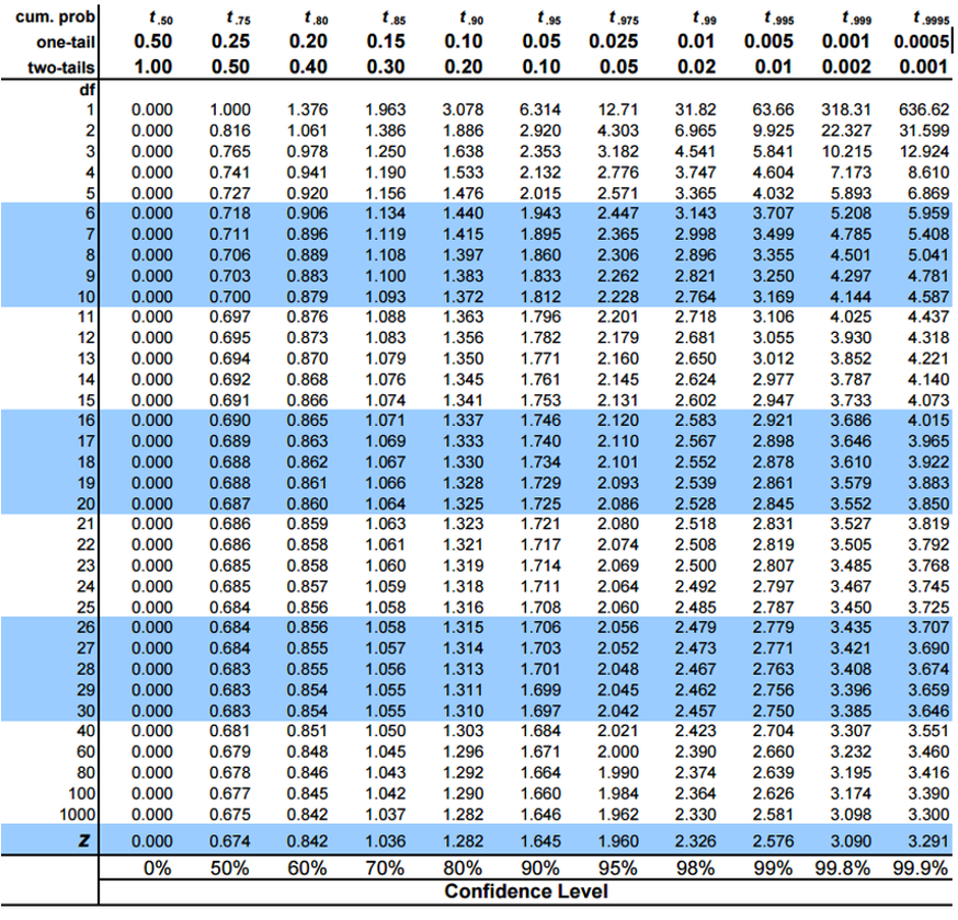

Worked CI — by table and by R

A sample of 9 fish: mean = 272.8, s = 37.81

1. df = 9 − 1 = 8
2. Two-tail 0.05 column, row 8 → t = 2.306
3. SE = 37.81 / √9 = 12.60
4. Margin = 2.306 × 12.60 = 29.06
5. CI = 272.8 ± 29.06 = 243.7 to 301.9 mm

“The 95% CI for mean length is 243.7–301.9 mm.”

Had we wrongly used 1.96, we’d have reported ±24.7 — an interval 15% too narrow, claiming precision we never had.

Practice 2 · z vs t on a real sample

Tip

Ten fish from I3. Same mean, same SE — only the multiplier differs.

set.seed(42)
small_sample <- i3_df %>% slice_sample(n = 10)
s_mean <- mean(small_sample$length_mm)
s_se   <- sd(small_sample$length_mm) / sqrt(10)

tibble(method = c("z (wrong)", "t (correct)"),
       crit  = round_half_up(c(1.96, qt(0.975, 9)), 3),
       lower = round_half_up(s_mean - crit * s_se, 1),
       upper = round_half_up(s_mean + crit * s_se, 1))

# A tibble: 2 × 4
  method       crit lower upper
  <chr>       <dbl> <dbl> <dbl>
1 z (wrong)    1.96  237.  280.
2 t (correct)  2.26  234.  284.

R agrees:

t.test(small_sample$length_mm)$conf.int

[1] 234.0564 283.7436
attr(,"conf.level")
[1] 0.95

The t interval is wider — and that extra width is the honest cost of not knowing σ.

Part 5 · Hypothesis testing

The logic

A confidence interval asks where is μ? A hypothesis test asks is μ equal to some specific value? Same machinery, different question.

1. H₀ — the boring claim: no effect, no difference
2. Hₐ — what we suspect instead
3. Assume H₀ is true and ask: how likely is data like ours?
4. p-value — probability of our result, or more extreme, if H₀ is true
5. α — how rare is rare enough, set before looking. Usually 0.05
6. Decide — p < α → reject H₀

\(t = \frac{\bar{y} - \mu_0}{s / \sqrt{n}}\) — how many SEs is our mean from the claim?

Note

📖 Reference

Whitlock & Schluter Ch. 6 — Hypothesis Testing.
Gotelli & Ellison Ch. 4 — Framing and Testing Hypotheses.

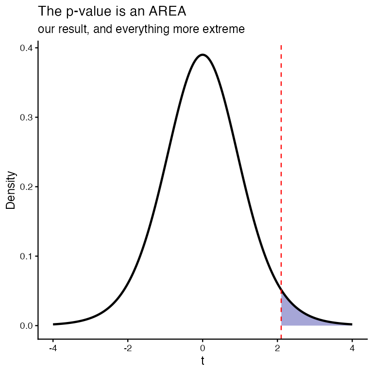
One-tailed: all of α at one end

Use when the question has a direction: are these fish longer than 285 mm? A shorter result would not interest us — it goes with H₀.

• H₀: μ ≤ 285 · Hₐ: μ > 285
• n = 20, so df = 19
• All 5% sits in the upper tail
• t-table, one-tail 0.05, row 19 → t = 1.729

Reject H₀ only if our t exceeds +1.729.

qt(0.95, df = 19)     # one-tailed, α = 0.05

[1] 1.729133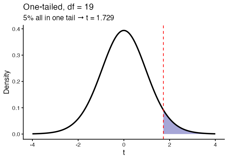

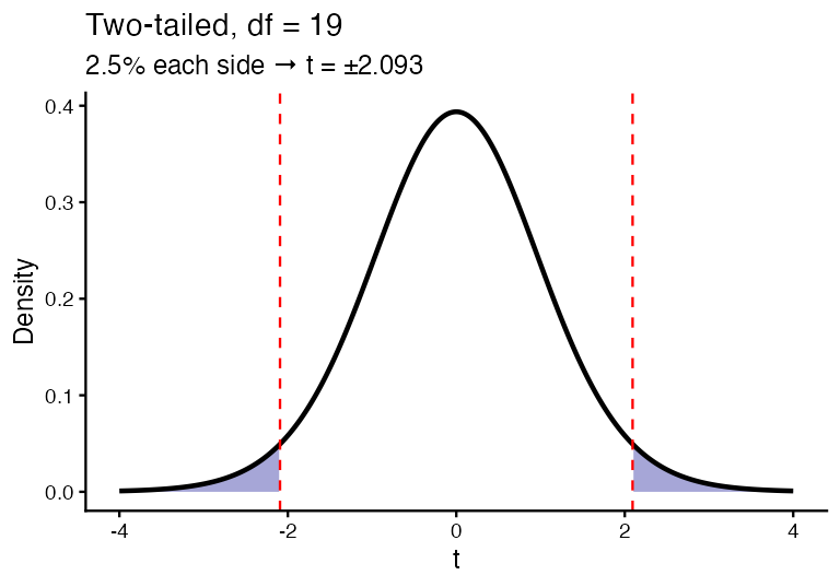
Two-tailed: α split between both ends

Use when either direction would matter: do these fish differ from 285 mm? Longer or shorter, we want to know.

• H₀: μ = 285 · Hₐ: μ ≠ 285
• Same df = 19, same total α = 0.05
• But now 2.5% in each tail
• t-table, two-tail 0.05, row 19 → t = 2.093

qt(0.975, df = 19)    # two-tailed, α = 0.05

[1] 2.093024

Important

Same α, same df, bigger critical value (2.093 > 1.729) — splitting α pushes each cutoff further out, so a two-tailed test is harder to pass.

Pick your tails from the question, before seeing the data. When in doubt, two-tailed — it is also R’s default.

Practice 3 · One-sample t-test

Tip

Are I3 grayling different from a historical mean of 260 mm?

H₀: μ = 260 · Hₐ: μ ≠ 260

t.test(i3_df$length_mm, mu = 260)

    One Sample t-test

data:  i3_df$length_mm
t = 1.6091, df = 65, p-value = 0.1124
alternative hypothesis: true mean is not equal to 260
95 percent confidence interval:
 258.6481 272.5640
sample estimates:
mean of x 
 265.6061 

Read the output in this order:

1. t — how many SEs from 260 we landed
2. df — n − 1
3. p-value — compare to α = 0.05
4. conf.int — and notice: does it contain 260? The CI and the test always agree

Practice 4 · Two-sample t-test

Tip

Are I8 fish longer than I3 fish? Directional → one-tailed.

t.test(length_mm ~ lake, data = grayling_df, alternative = "less")

    Welch Two Sample t-test

data:  length_mm by lake
t = -15.532, df = 161.63, p-value < 2.2e-16
alternative hypothesis: true difference in means between group I3 and group I8 is less than 0
95 percent confidence interval:
      -Inf -86.66138
sample estimates:
mean in group I3 mean in group I8 
        265.6061         362.5980 

lake is alphabetical, so R tests I3 − I8. “I8 longer” therefore means I3 − I8 is less than zero → alternative = "less".

Note “Welch Two Sample t-test” — R does not assume the two lakes have equal variances, and here that matters: sd(I3) = 28.3 mm but sd(I8) = 52.3 mm.

What a p-value is not

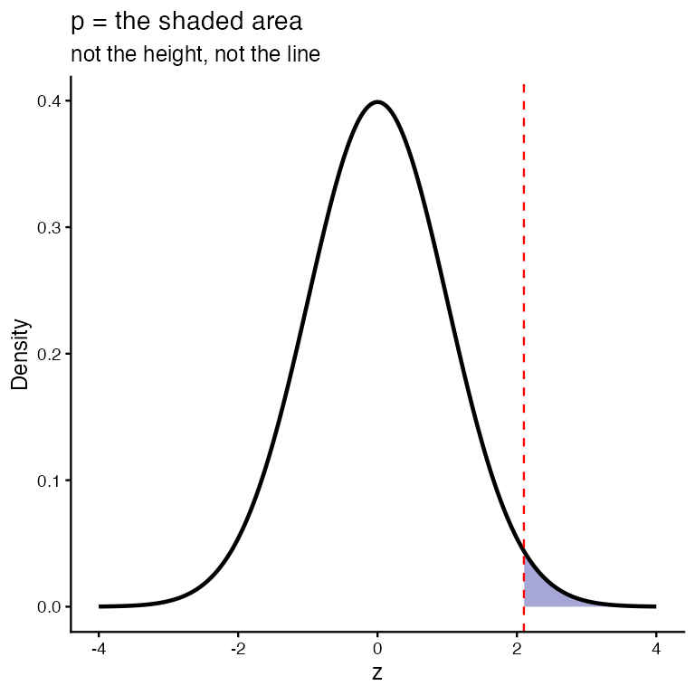
It is: the probability of data like ours if H₀ were true.

It is not:

• the probability that H₀ is true
• the probability the result is due to chance
• a measure of how big the effect is

Small p means detectable, not large. With n = 168, a biologically meaningless 2 mm difference can return p = 10⁻¹⁶.

So, every time:

• report p < 0.001, not p = 1.2e-16
• report the effect size — the difference in millimetres
• report the CI — it shows size and uncertainty in one line
• significant ≠ important. That call is biology, not arithmetic

Note

📖 Reference

Gotelli & Ellison Ch. 4 — “Statistical Significance and P-Values.”

Summary

The chain, end to end:

1. Data have a distribution — μ and σ describe a normal one
2. z = (x − μ)/σ collapses every normal curve onto one standard curve
3. Area under that curve is probability — pnorm for areas, qnorm for cutoffs
4. All of it assumes normality. Shapiro-Wilk plus a Q-Q plot; our fish failed, and the tail was off by a third
5. SD describes fish; SE = s/√n describes means. Never swap them
6. CI = ȳ ± t · SE — 95% of intervals built this way capture μ
7. σ is never known, so the multiplier is t, not 1.96 — fatter tails, wider interval, honest
8. A p-value is tail area under H₀. It measures detectability, never importance

Note

Up next — t-Tests, then Power and Error, where Type I/II errors and statistical power get the full treatment they need.

Readings

Before next class — chapter PDFs are on Canvas:

• Whitlock & Schluter — Ch. 10, The Normal Distribution; Ch. 4, Estimating with Uncertainty; Ch. 11, Inference for a Normal Population. If you read only one, read Ch. 4
• Gotelli & Ellison — Ch. 2, Random Variables and Probability Distributions; Ch. 4, Framing and Testing Hypotheses

Today’s topic	Read
Normal distribution, z-scores	W&S Ch. 10
Checking normality	W&S Ch. 13
SE and confidence intervals	W&S Ch. 4
The t-distribution	W&S Ch. 11
Hypothesis tests, p-values	W&S Ch. 6; Gotelli Ch. 4

Note

📖 R for Data Science (2e)

• §9 — Layers
• §10 — Exploratory data analysis
• §13 — Numbers