Spatial data, sf, and geom_sf with real Bigfoot sighting reports
maps
sf
spatial
ggplot
A 2-day intro to maps in R. Spatial data and coordinate systems, the sf package, turning latitude/longitude into a map with geom_sf(), drawing points on US states, and building a per-state choropleth by joining counts to the map — all with ~4,600 real Bigfoot sighting reports.
Author
Bill Perry
Published
October 5, 2026
Where we left off — Factors & Joins
Factors — reordered and relabeled categories for readable plots
Joins — combined a measurements table with a second table by a shared key
Both skills come back today: we’ll join sighting counts onto a map
Note
✅ Transition
You can wrangle, summarize, model, and join — today those skills point at a map instead of a table. Our dataset: ~4,600 real Bigfoot sightings across the US, each with a latitude and longitude, ready to become points and then a choropleth. 🦶
Goals for today (a 2-day lecture)
Understand spatial data — points, polygons, and coordinate systems
Meet sf — a data frame with a geometry column
Turn latitude/longitude into a map with geom_sf()
Draw sighting points on a map of US states
Build a choropleth — sightings per state — by joining counts to the map
Reproject to a proper US look
Tools today:
tidyverse, sf, maps
Data:
bfro_reports_geocoded.csv from Kaggle — save it to your data/ folder
Day 1: points on a map. Day 2: choropleth + polish.
How to Use These Slides — Predict · Type · Run
This lecture runs in four chunks over two days. After each chunk you switch to the activity and type the code yourself.
For every map, do three things:
Predict — before it draws, say where the points or the dark states will be
Type the code by hand — do not copy-paste
Run it and compare to your prediction
Note
✅ Why bother?
Naming the state you expect to be darkest before it renders is what makes you look at the result instead of admiring it.
st_as_sf(coords = ..., crs = ...) and geom_sf() have a specific argument order — typing them is what makes it stick.
Spatial objects, basemaps, joins and projections each get their own chunk, so a CRS mismatch doesn’t get confused with a join-key mismatch.
🧩 Chunk 1 of 4 · Spatial Data & the sf Object (Day 1)
We will cover: what spatial data is, coordinate systems, and turning latitude/longitude into an sf object.
Tip
🖐 After this chunk: Activity Parts 1–3 (load the sightings, make them spatial).
What Is Spatial Data?
Two shapes cover almost everything:
Points — a single location: one Bigfoot sighting = (longitude, latitude)
Polygons — an area: the outline of a state or country
Both need a coordinate reference system (CRS) — the rulebook that says what the numbers mean.
EPSG:4326 (WGS84) — plain longitude/latitude, what GPS and our CSV use
Note
📖 New word
CRS = Coordinate Reference System. Two maps won’t line up unless they share one. Lat/long is crs = 4326.
The sf Package — a Data Frame with Geometry
# Load packages + the sighting data ------------------library(tidyverse)library(sf) # simple features = spatial data frameslibrary(maps) # ready-made state/country outlines# Swap this path for your download -------------------bigfoot_df <-read_csv("data/bfro_reports_geocoded.csv")bigfoot_df %>%select(title, state, latitude, longitude, classification) %>%head()
# A tibble: 6 × 5
  title                   state latitude longitude classification
  <chr>                   <chr>    <dbl>     <dbl> <chr>
1 <NA>                    Alab…     NA        NA   Class B
2 <NA>                    Alas…     NA        NA   Class A
3 Report 6496: Bicycling… Rhod…     41.4     -71.5 Class A
4 <NA>                    Penn…     NA        NA   Class B
5 <NA>                    Oreg…     NA        NA   Class B
6 Report 9765: Motorist … Okla…     35.3     -99.2 Class A
sf = “simple features” — the standard for spatial data in R
An sf object is a normal tibble plus a geometry column
Everything you know — filter(), mutate(), group_by() — still works
Clean the Coordinates First
# Drop missing coords + keep the lower 48 ------------bigfoot_df <- bigfoot_df %>%filter(!is.na(latitude), !is.na(longitude)) %>%filter(longitude >-125, longitude <-66, latitude >24, latitude <50)nrow(bigfoot_df)
[1] 4031
Real coordinate data always has some missing values
We also trim to the continental US so the map isn’t dominated by a few far-flung points
Warning
⚠️ Watch out! The next step (st_as_sf) errors if any latitude/longitude is NA — clean first, always.
Make It Spatial — st_as_sf()
Note
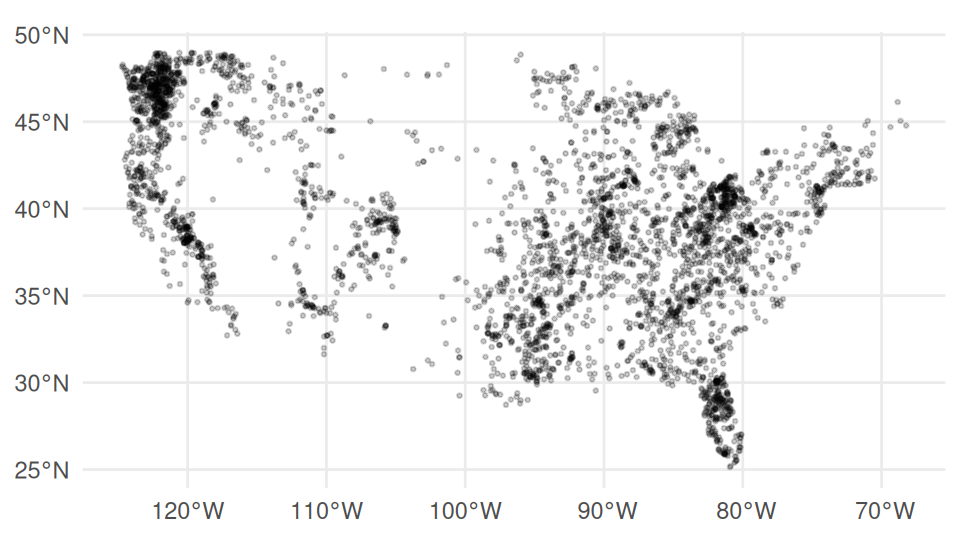
🔮 Predict first: ~4,600 rows of lat/long, plotted with no basemap. What shape will the cloud of points make?
# Build the geometry column from lon/lat -------------bigfoot_sf <- bigfoot_df %>%st_as_sf(coords =c("longitude", "latitude"), crs =4326)# Just the points — the USA appears on its own -------ggplot(bigfoot_sf) +geom_sf(alpha =0.2, size =0.5) +theme_minimal()
coords = c("longitude", "latitude") — x first, then y
crs = 4326 — tells sf these are lon/lat degrees
The points alone trace the outline of the country — that’s the “aha” of spatial data
📖 sf: st_as_sf()
🛑 Pause — Do Activity Parts 1–3 Now
Load the sightings, clean the coordinates, make an sf object, and plot the bare points. Predict the shape before you run it.
🧩 Chunk 2 of 4 · Points on a Real Map (Day 1)
We will cover: adding a basemap of US states and layering the sightings on top, colored by class.
Tip
🖐 After this chunk: Activity Parts 4–6 (draw the states + points).
Get a Basemap — US States as sf
# Turn the built-in state outlines into sf ----------states_sf <-st_as_sf( maps::map("state", plot =FALSE, fill =TRUE)) %>%st_set_crs(4326)states_sf %>%head(3)
Simple feature collection with 3 features and 1 field
Geometry type: MULTIPOLYGON
Dimension:     XY
Bounding box:  xmin: -114.8093 ymin: 30.24071 xmax: -84.90089 ymax: 37.00161
Geodetic CRS:  WGS 84
               ID                           geom
alabama   alabama MULTIPOLYGON (((-87.46201 3...
arizona   arizona MULTIPOLYGON (((-114.6374 3...
arkansas arkansas MULTIPOLYGON (((-94.05103 3...
maps::map("state", fill = TRUE) — polygon outlines of the lower 48, no download
st_as_sf() converts them to spatial features
st_set_crs(4326) — same lat/long system as our points, so they line up
Note
The ID column holds the state name (lowercase) — we’ll use it to join later.
Layer the Sightings on the Map
Note
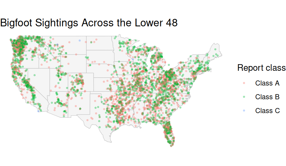
🔮 Predict first: Densest cluster — Pacific Northwest, Southeast, or Plains? Commit before it draws.
# Basemap first, then points on top ------------------ggplot() +geom_sf(data = states_sf, fill ="grey96", color ="grey75") +geom_sf(data = bigfoot_sf, aes(color = classification),alpha =0.3, size =0.6) +labs(title ="Bigfoot Sightings Across the Lower 48",color ="Report class") +theme_void()
Order matters: draw states first, points second (on top)
aes(color = classification) — colors Class A / B / C reports
theme_void() — drop the axes and grid for a clean map
Notice the clusters — the Pacific Northwest lights up. 👀
🛑 End of Day 1 · Start Day 2 Here
Day 1 recap — you can now:
Explain points, polygons, and CRS
Turn lat/long into an sf object with st_as_sf()
Draw a basemap of states and layer points with geom_sf()
Day 2 — the choropleth:
Count sightings per state
Join those counts onto the map
Shade each state, then reproject for a proper US look
🧩 Chunk 3 of 4 · Choropleth by State (Day 2)
We will cover: counting sightings per state and joining them to the map to shade each state.
Tip
🖐 After this chunk: Activity Parts 7–9 (count, join, shade).
Step 1 — Count Sightings per State
Note
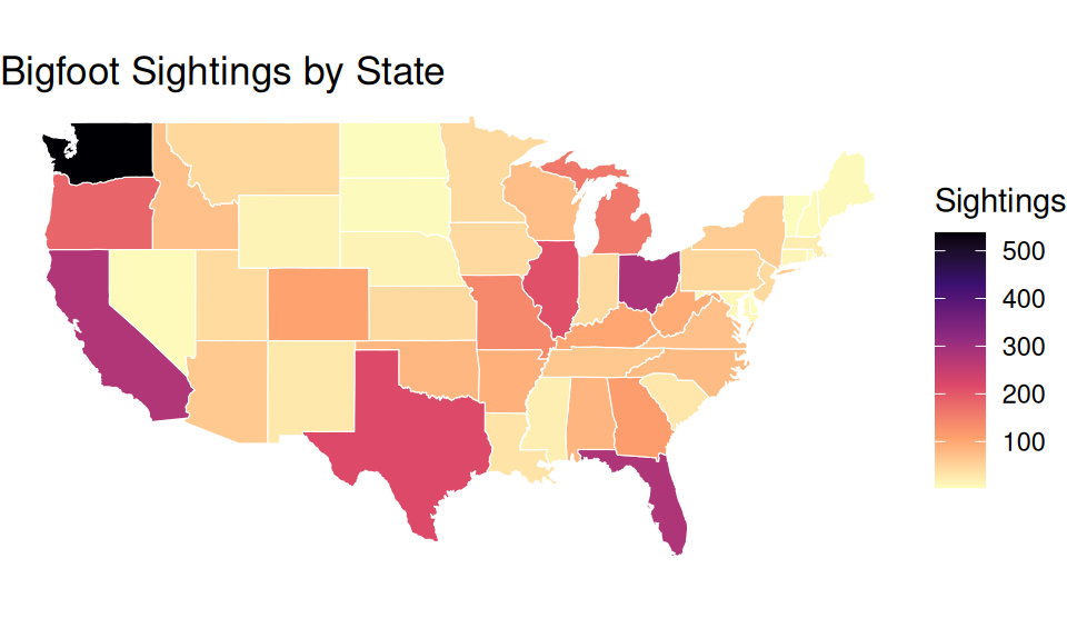
🔮 Predict first: Which state do you think has the most Bigfoot reports? Write your guess before you run count().
# Sightings per state — lowercase to match the map --sightings_by_state <- bigfoot_df %>%mutate(state =str_to_lower(state)) %>%count(state, name ="sightings") %>%arrange(desc(sightings))head(sightings_by_state)
# A tibble: 6 × 2
  state      sightings
  <chr>          <int>
1 washington       538
2 ohio             283
3 florida          281
4 california       277
5 texas            218
6 illinois         210
count(state) — one row per state with its total
str_to_lower(state) — the map’s state names are lowercase, so we match them now
This is a plain summary table — next we glue it to the geometry
📖 R4DS §16 — factors/strings for tidy keys
Live Demo — Watch It Break (a blank map)
If I skip the lowercase step, the join keys don’t match — "Washington" ≠ "washington":
states_sf %>%mutate(state = ID) %>%# "Washington" vs "washington"left_join(count(bigfoot_df, state), by ="state")
Every state gets NA sightings → the whole map renders grey. No error, just a blank choropleth.
The fix — make both keys the same case before joining (str_to_lower()).
Important
✅ Why show a blank choropleth?
left_join() doesn’t know that "Washington" and "washington" mean the same state — as far as R is concerned they’re two unrelated strings, so every row fails to match and sightings comes back NA everywhere. scale_fill_viridis_c() then has nothing to shade with, and you get a map that ran without a single error yet shows you nothing. Grey-everywhere is the signature of a key-mismatch, not a code bug.
Step 2 — Join Counts onto the Map
# Join sightings to the state polygons ---------------states_map <- states_sf %>%# drop ":north" etc.mutate(state =str_remove(ID, ":.*")) %>%left_join(sightings_by_state, by ="state")ggplot(states_map) +geom_sf(aes(fill = sightings), color ="white") +scale_fill_viridis_c(option ="magma", direction =-1) +labs(title ="Bigfoot Sightings by State",fill ="Sightings") +theme_void()
left_join() keeps every state, filling in its count
scale_fill_viridis_c() — a colorblind-safe gradient
This is a choropleth — the map is the bar chart.
🛑 Pause — Do Activity Parts 7–9 Now
Count sightings per state, join them to the map, and shade the choropleth. Predict the top state before you run it.
🧩 Chunk 4 of 4 · Polish & Explore (Day 2)
We will cover: a proper US projection, and a fun exploration — sightings by season.
Tip
🖐 After this chunk: Activity Parts 10–12 (reproject, then explore).
Reproject for a Proper US Look — coord_sf()
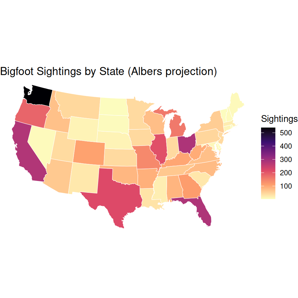
# Albers Equal-Area (EPSG:5070) — the "textbook" US --ggplot(states_map) +geom_sf(aes(fill = sightings), color ="white") +scale_fill_viridis_c(option ="magma", direction =-1) +coord_sf(crs =5070) +labs(title ="Bigfoot Sightings by State (Albers projection)",fill ="Sightings") +theme_void()
Lat/long (4326) stretches the US; Albers (5070) is the shape you expect
coord_sf(crs = 5070) reprojects just for display — your data is unchanged
One line, and the map suddenly looks professional
Note
Different jobs use different CRSs — equal-area for choropleths, web maps use 3857.
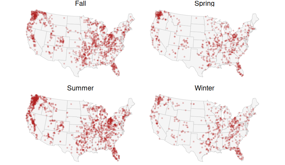
Explore — Sightings by Season 🍂
Note
🔮 Predict first: In which season do you think the most sightings are reported? (Think about who is outdoors, and when.)
# Facet the point map by season ----------------------bigfoot_sf %>%filter(season %in%c("Spring","Summer","Fall","Winter")) %>%ggplot() +geom_sf(data = states_sf, fill ="grey96", color ="grey80") +geom_sf(alpha =0.2, size =0.4, color ="firebrick") +facet_wrap(~ season) +coord_sf(crs =5070) +theme_void()
facet_wrap(~ season) — one small map per season, same skill as any facet
Summer dominates — more people outdoors = more reports (a sampling story!)
This is how you’d explore any point dataset: filter, color, facet
What We Learned Today
Concepts:
Spatial data = points/polygons + a CRS
sf objects are tibbles with a geometry column
st_as_sf(coords = c("lon","lat"), crs = 4326) makes points
geom_sf() draws layers; order matters (basemap first)
A choropleth = counts joined to polygons, shaded by value
coord_sf(crs = ...) reprojects for display
R skills:
st_as_sf(), st_set_crs(), maps::map()
geom_sf(), scale_fill_viridis_c(), coord_sf()
count() + left_join() + str_to_lower() for the choropleth