Lecture 02 — Introduction to R and Positron

R, Positron and Projects

How to we make projects that are repeatable and organize the chaos into structure and how to use R and Posiotron.

Author

Bill Perry

Published

July 5, 2026

Where we left off (Lecture 01)

Science fundamentals — falsifiable predictions; null vs. alternate hypotheses
Our class project — leaf morphology: sunny vs. shady sides of trees
Design — randomization, replication (multiple trees), sampling limits
Variables — dependent (leaf mass/size) vs. independent (side of tree)
Spreadsheet hygiene — metadata, consistent column names, units, clean sheet design
Installed R and Positron before today

Note

✅ Key idea

Today we take that tidy spreadsheet and bring it to life in R.

Goals for today

Get R and Positron oriented — the four panes
Organize a project so future-you can find things
Learn how R actually works:
- using it as a calculator
- storing things with <- the assignment operator - alligator eats the minus sign…
- values, vectors, and data types
- writing a script
Load our tree data and make a first plot

Tip

🖐 Try it yourself

By the end you will run real code on our leaf data — not a toy dataset.

Part 1 · Setting up

What is R, really?

R is the engine — a free language for data and statistics
We drive that engine through an IDE (a code editor)
Two good IDEs — you may try both:
- Positron — what we use (recommended)
- RStudio — the long-time classic

Note

📖 New word

IDE = Integrated Development Environment. Think of R as the car engine and the IDE as the seat, wheel, and dashboard.

Organize the project before you code

Make one folder per project. Everything for the tree experiment lives together:

tree_project/
├── data/          ← your Excel and CSV files
├── scripts/       ← your .R code files
└── figures/       ← plots you save

In Positron: File → Open Folder… and pick this folder
Every path is then relative to the project — no more C:/Users/.../Desktop/... nightmares

Note

✅ Key idea

A tidy folder today saves an hour of “where did I put that file?” next week.

Note

📊 Coming from Excel?

In Excel you keep one big file and it can be hard to figure out what was done and how
In R we keep raw data untouched and
- write new processed files
  - — so you can always trace your steps and never overwrite your original numbers

A quick tour of Positron

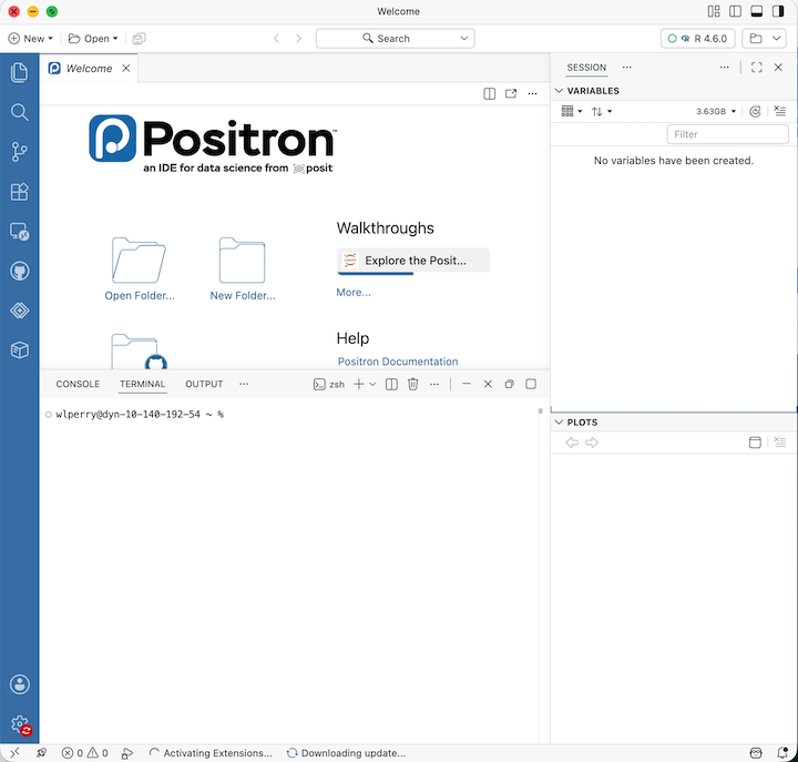
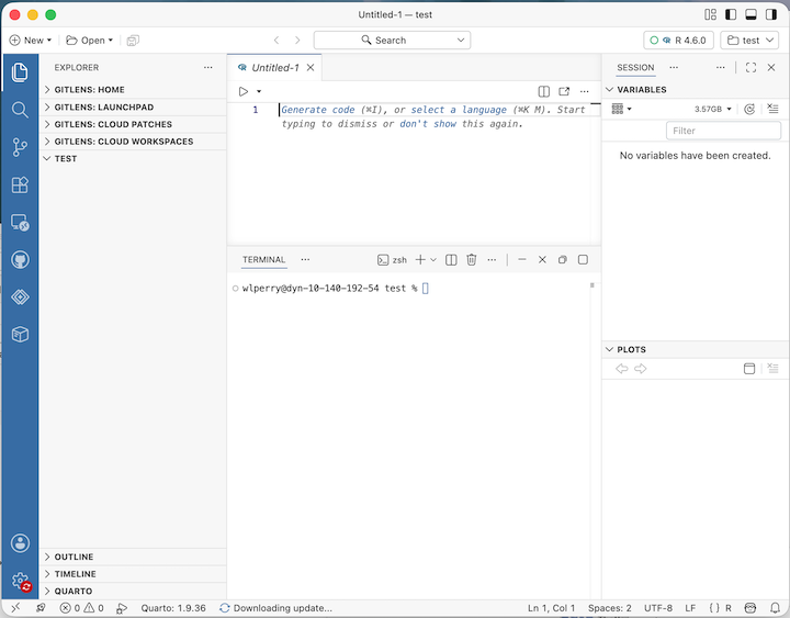
Four panes you will use constantly:

Editor (top-left) — your scripts live here when you have a script open
Console / Terminal (bottom) — where code runs
Variables / Session (right) — everything you have stored
Plots (right) — your figures appear here

Tip

🖐 Try it yourself

Find each pane on your screen now.
Click the Console tab — that is where we start next.

Part 2 · How R works

R is a calculator

Type math straight into the console and press Enter:

3 + 5
12 / 7
2 ^ 10

R answers immediately. The console is great for quick “what is the answer?” questions.

Warning

⚠️ Watch out!

A + at the start of the console line means R is still waiting for you to finish a command. Press Esc to start over.

Note

📊 Coming from Excel?

This is just like typing =3+5 into an Excel cell — except there are no cells, just a line you type and run.

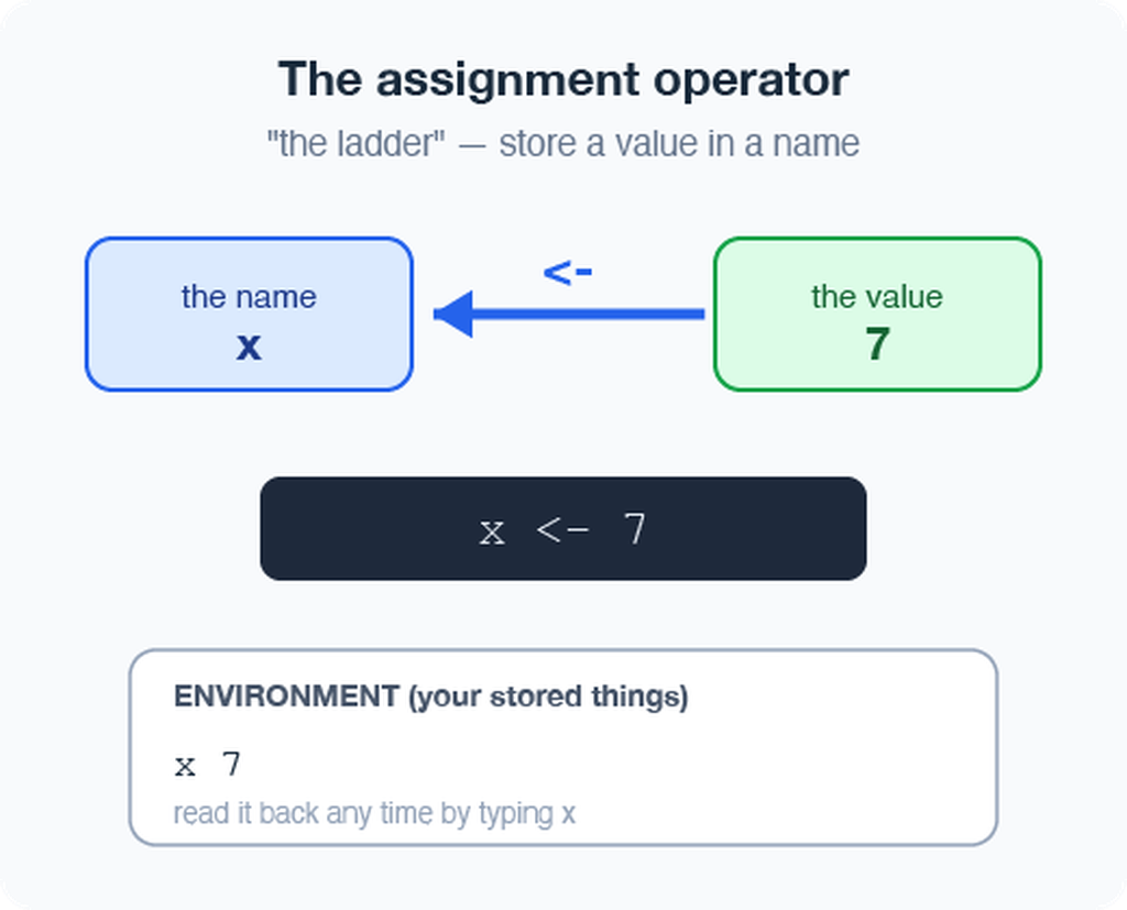
Storing values with `<-` assignment operator - alligators eats minus sign

To keep a value, give it a name with the assignment operator <-:

x <- 7          # store 7 under the name x
x               # type the name to read it back
x * 2           # use it in math

<- puts the value into your environment (look in the Variables pane!)
Shortcut: Alt + - (Win) or Option + - (Mac) types <- for you

Note

📖 New word

Assignment operator <- “puts the thing on right and stores it in the name on left.” not always the same as =

Naming your objects well

Good names make code readable months later:

Be explicit, not too long: leaf_mass, not x2
Cannot start with a number — x2 ✅, 2x ❌
R is case-sensitive — weight_g ≠ Weight_g
Use lower_snake_case — words separated by underscores

leaf_mass   <- c(4, 3, 5, 7)   # good
LeafMass    <- c(4, 3, 5, 7)   # works but avoid
leaf.mass   <- c(4, 3, 5, 7)   # avoid dots

Warning

⚠️ Watch out!

weight_g and weight_G are two different objects. Pick one style and stick with it. I URGE you to use lower case and _

Note

📖 New word

Object (R) = variable (Excel/other languages). Same idea: a named container that holds something.

Our naming convention throughout this course:
- - data frames → _df
- - plots → _plot
- - models → _model

Leave notes with comments `#`

Anything to the right of # is ignored by R — it is a note for humans:

# weights of four leaves, in grams
leaf_mass <- c(4, 3, 5, 7)

mean(leaf_mass)   # average leaf mass

Comment generously — your future self will thank you
Shortcut to toggle: Ctrl/Cmd + Shift + C

Note

✅ Key idea

If a line confused you while writing it, comment why you did it.

Note

📊 Coming from Excel?

Comments are like the notes you scribble in a cell — but they never get in the way of the numbers or the code.

Functions and their arguments

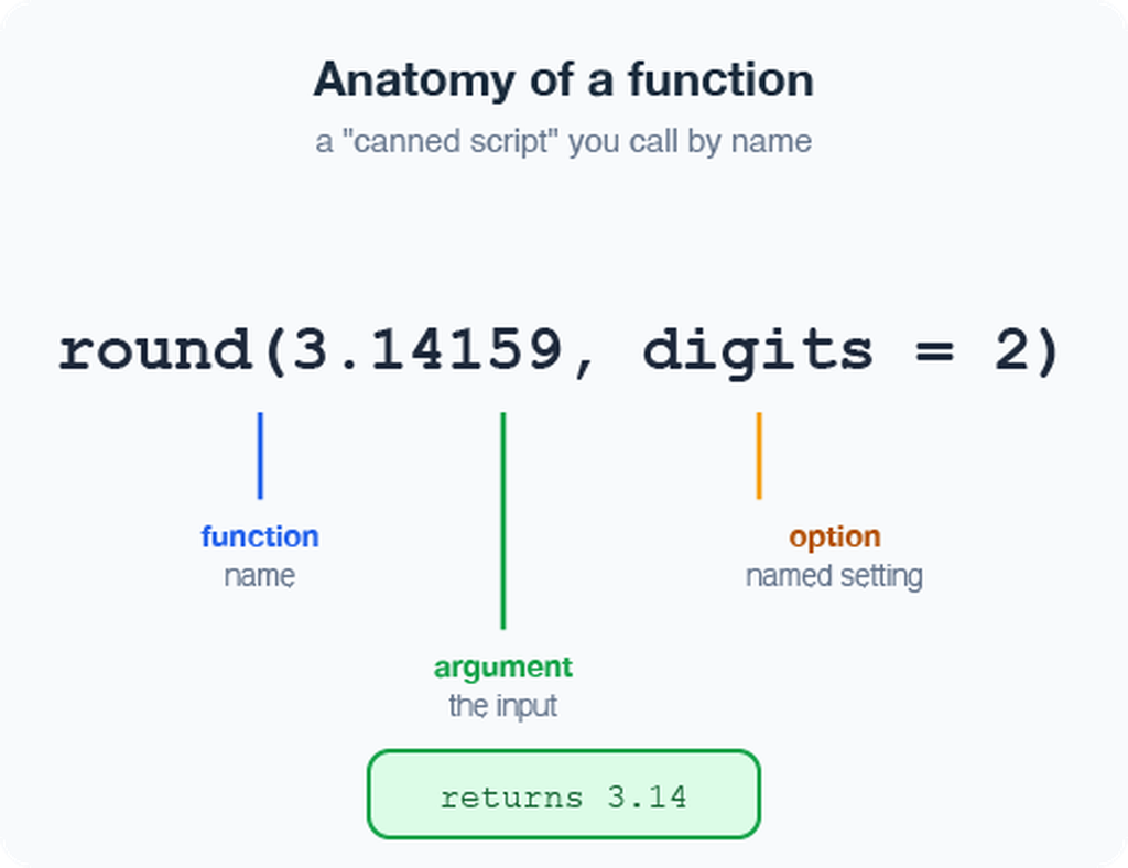
A function is a canned script you call by name. You feed it arguments (inputs); it returns a result:

sqrt(10)                         # one argument
round(3.14159)                   # default: 0 digits → 3
round(3.14159, 2)                # two digits → 3.14
round(x = 3.14159, digits = 2)  # named arguments

Stuck on a function?

?round        # open the help page
args(round)   # what arguments does it take?

Note

📖 New word

Argument = an input you hand to a function inside its ( ).

Vectors — a row of values

A vector is a series of values built with c() (“combine”) or concatenated list:

weight_g <- c(4, 3, 5, 7)          # numbers
side     <- c("sunny", "shady")     # text needs quotes

Inspect any vector:

length(weight_g)   # how many values?
class(weight_g)    # what type?
str(weight_g)      # quick structure overview

Warning

⚠️ Watch out!

Quotes matter: "sunny" is text. Without quotes, R hunts for an object named sunny and errors when it cannot find one.

Note

✅ Key idea

A vector is the workhorse of R. A spreadsheet column is really just a vector.

Data types live inside vectors

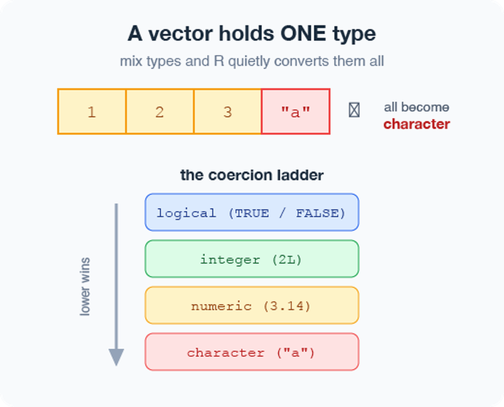
Every vector holds one type:

numeric — 4, 3.5
character — "sunny"
logical — TRUE / FALSE

Mix types and R quietly coerces them all to one:

c(1, 2, 3, "a")     # all become character
c(1, 2, 3, TRUE)    # TRUE becomes 1
class(c(1, 2, 3, "a"))

Note

📖 New word

Coercion = R automatically converting everything in a vector to a single shared type.

Part 3 · From console to script

Do not retype — use a script

The console forgets.

A script (.R file) remembers and re-runs.

File → New File → R File opens a blank script
Type your commands, one per line
Put the cursor on a line and press Ctrl/Cmd + Enter to run it
Save with Ctrl/Cmd + S — reopen later and re-run everything

x    <- 7
y    <- 5
x + y

Note

✅ Key idea

Console = scratch paper.
Script = the lab notebook you keep.

Packages — extending what R can do

Like apps for your phone, packages add new abilities to R.

Install once — downloads to your computer (do this in the Console, not in your script):

install.packages("tidyverse")
install.packages("readxl")

Load every session — activates it for today (put this at the top of every script):

library(tidyverse)   # data wrangling + plotting
library(readxl)      # read Excel files

Warning

⚠️ Watch out!

If R says “could not find function read_excel”, you forgot the library(readxl) line.

Note

📖 New words

Package = the installed toolbox (install once).

Library = loading that toolbox into today’s session (every session).

Part 4 · Loading our data

Two functions for two file types

Put your files in the project’s data/ folder, then:

library(tidyverse)
library(readxl)

# Excel files (.xlsx)
tree_df <- read_excel("data/2026_06_25_tree_experiment_raw_data.xlsx")

# CSV files (.csv) — used by NOAA, iNaturalist, many databases
noaa_df <- read_csv("data/noaa_global_yearly_temps.csv")

Note

✅ Key idea

read_excel() needs library(readxl). read_csv() comes with library(tidyverse) — no extra install needed.

Note

📊 Coming from Excel?

read_excel() and read_csv() are the bridge from your file into R. Your file’s first row becomes the column names in R.

Meet the data frame

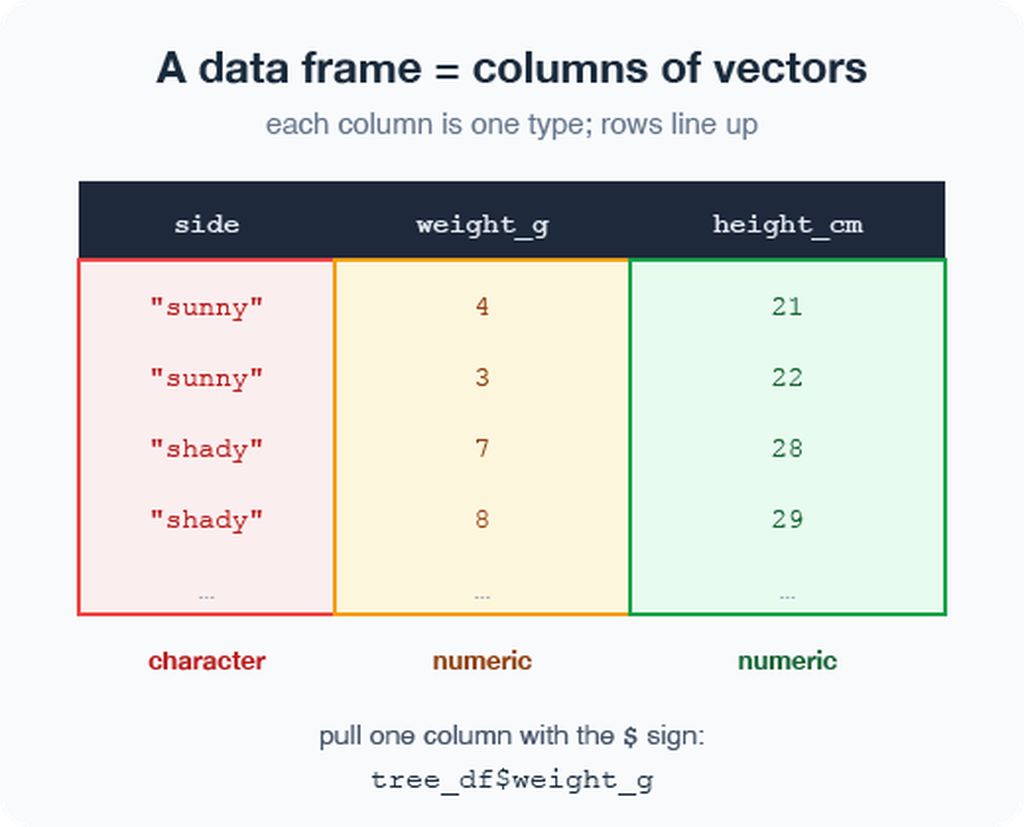
A data frame is a table: each column is a vector of one type, and the rows line up.

Our tree_df has five columns:

index — leaf number (numeric)
side — "sunny" / "shady" (character)
weight_g, width_cm, height_cm (numeric)

Pull a single column with $:

tree_df$weight_g     # just the weights, as a vector

Note

📖 New word

Data frame = R’s word for a spreadsheet-style table.

Look at your data before trusting it

Always eyeball a new data frame:

head(tree_df)      # first 6 rows
tail(tree_df)      # last 6 rows
dim(tree_df)       # rows, columns  → 20  5
names(tree_df)     # column names

# Tidyverse-style structure check (prefer this over str):
glimpse(tree_df)   # one line per column: name, type, first values

# Base R equivalent:
str(tree_df)       # same information, different layout

Tip

🖐 Try it yourself

Run glimpse(tree_df). How many rows? What type is side?

Note

✅ Key idea

Check dim() and glimpse() every single time you load data. Typos and wrong column types hide here.

Warning

⚠️ Watch out!

If a number column shows as <chr>, a stray letter or comma snuck into your spreadsheet.

The pipe `%>%` — read it as “then”

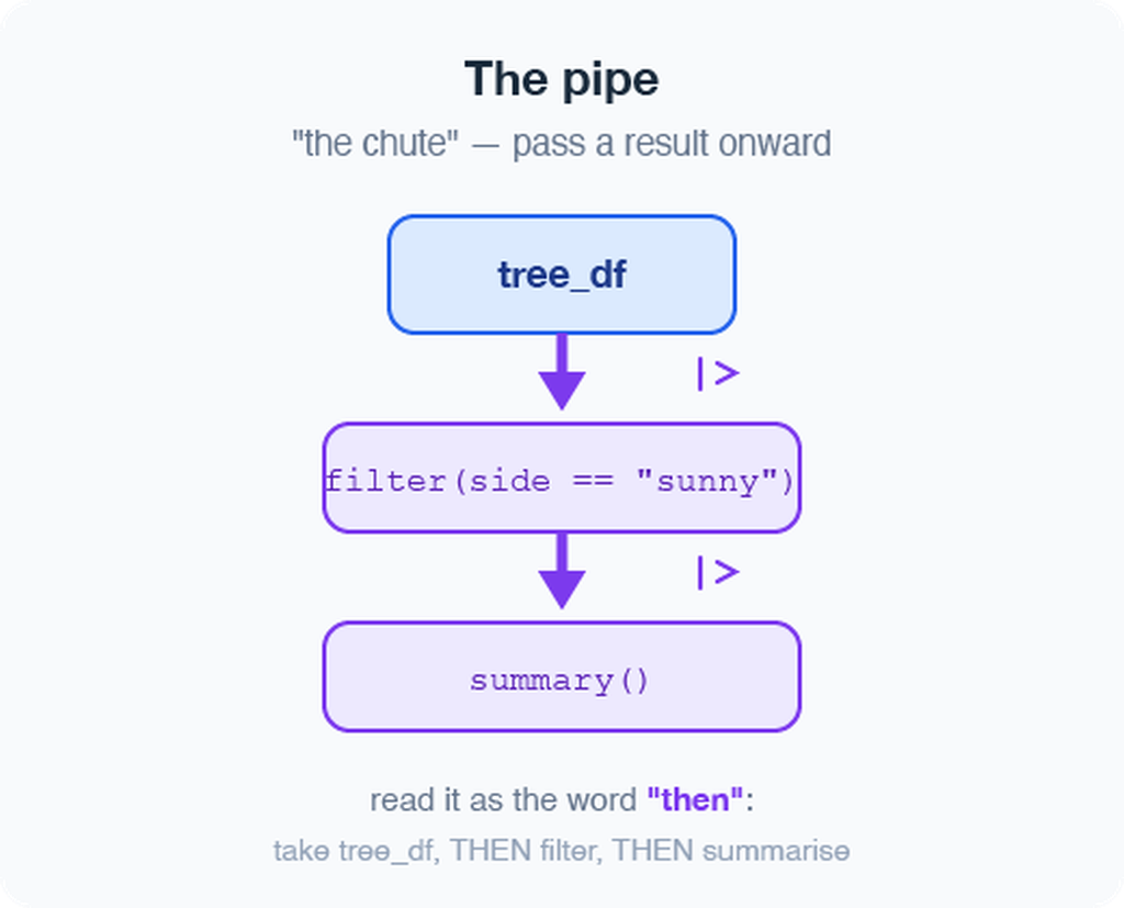
The pipe sends a result straight into the next function. Read %>% as the word “then”:

# Start with simple examples:
tree_df %>% nrow()         # take tree_df, THEN count rows
tree_df %>% names()        # take tree_df, THEN list column names
tree_df %>% summary()      # take tree_df, THEN summarize

# Chain two steps:
tree_df %>%
  head(3)                  # take tree_df, THEN show first 3 rows

In Lecture 03 we will chain more steps together.

Note

📖 New word

Pipe %>% = “take what is on the left and feed it to the function on the right.”

Note

Two pipes — same idea:

%>% — from tidyverse (we use this one)
|> — built into R 4.1+ (the “native pipe”)
They behave identically for everything in this course.

Part 5 · Your first plot

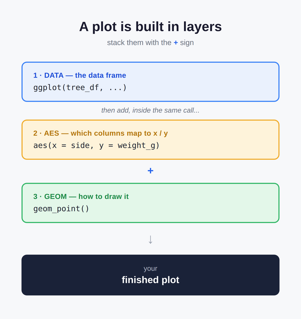
ggplot: build a picture in layers

Plots are built from three core pieces, joined with +:

ggplot(tree_df, aes(x = side, y = weight_g))

data — which data frame (tree_df)
aes — which columns map to x and y
geom — how to draw it (add with +)

ggplot(tree_df, aes(x = side, y = weight_g)) +
  geom_point()

Warning

⚠️ Watch out!

The + must sit at the end of a line, never the start.
+ at the start = error
AND YES - Totally confusing to have %>% for code and + for plots - but its the way it is….

Improve it one layer at a time

Since side is a category, a boxplot with the raw points on top tells the story well:

ggplot(tree_df, aes(x = side, y = weight_g)) +
  geom_boxplot() +
  geom_jitter(width = 0.15, alpha = 0.6, color = "tomato") +
  labs(x = "Side of tree",
       y = "Leaf weight (g)",
       title = "Sunny vs. shady leaves")

Tip

🖐 Try it yourself

Swap weight_g for height_cm. What changes? Try geom_violin() instead of geom_boxplot().

CAN YOU DRAW A SKETCH OF WHAT THIS MIGHT LOOK LIKE???

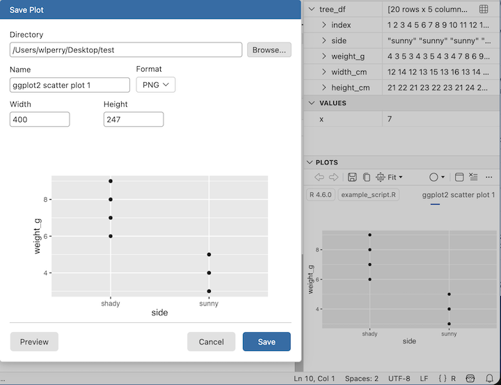
Save your plot and your script

Store the plot in an object, then save it as a PNG:

leaf_plot <- ggplot(tree_df, aes(x = side, y = weight_g)) +
  geom_boxplot()

# Save to the figures/ folder — always use PNG, dpi = 300
ggsave("figures/leaf_weight.png",
       plot   = leaf_plot,
       width  = 6,
       height = 6,
       units  = "in",
       dpi    = 300)

📖 File format tip
Save figures as PNG (.png) for reports and Canvas submissions.
dpi = 300 means 300 dots per inch — high enough for print and posters.

Warning

⚠️ Watch out!

ggsave() wants the filename first, then plot =. Also: dpi = 300 is publication quality — always use it.

Note

Wrap-up · What you can now do

Set up R + Positron and organize a project folder
Use R as a calculator and store values with <-
Write and run a script, with # comments
Call functions and read their help with ?
Build vectors, know their types
Load Excel and CSV data with read_excel() and read_csv()
Inspect a data frame with glimpse(), head(), dim()
Use the pipe %>% to chain steps
Make and save a first ggplot as a PNG

Tip

🖐 Before next class

Load tree_df, run glimpse(), and make one plot of width_cm by side. Save it to figures/.

Note

✅ Key idea

You went from a blank console to a saved figure of our data. That is the whole workflow in miniature.

Up next — Lecture 03:

filter() — pick rows
select() — pick columns
mutate() — create new columns
arrange() — sort rows
Then: descriptive statistics on our leaf data

Getting unstuck

When code breaks (it will — that is normal):

?function_name — the built-in help page
Read the error message out loud; it usually names the line
Check: did you load library(tidyverse) and library(readxl)?
Check: spelling? A missing ) or +?
The posit/tidyverse cheatsheets are excellent: posit.co/resources/cheatsheets
Bring the exact error (copy-paste it) to class or office hours

Note

✅ Key idea

Every coder googles error messages daily. Getting stuck is not failing — it is the job.

Note

📊 Coming from Excel?

In Excel you fix errors by clicking around. In R you fix them by reading the message and editing one line. Slower at first, far more powerful soon.

Other Formats

Where we left off (Lecture 01)

Goals for today

Part 1 · Setting up

What is R, really?

Organize the project before you code

A quick tour of Positron

Part 2 · How R works

R is a calculator

Storing values with <- assignment operator - alligators eats minus sign

Naming your objects well

Leave notes with comments #

Functions and their arguments

Vectors — a row of values

Data types live inside vectors

Part 3 · From console to script

Do not retype — use a script

Packages — extending what R can do

Part 4 · Loading our data

Two functions for two file types

Meet the data frame

Look at your data before trusting it

The pipe %>% — read it as “then”

Part 5 · Your first plot

ggplot: build a picture in layers

Improve it one layer at a time

Save your plot and your script

Wrap-up · What you can now do

Getting unstuck

Storing values with `<-` assignment operator - alligators eats minus sign

Leave notes with comments `#`

The pipe `%>%` — read it as “then”