Lecture 14 — One-Way ANOVA II: Running & Reporting the Test

Reading the F table, finding which groups differ, and writing it up

Running the one-way ANOVA with aov() and car::Anova(), finding WHICH penguin species differ with emmeans post-hoc tests, and writing a complete results sentence.

Where we left off (Lecture 13 — One-Way ANOVA I)

• mass_model <- lm(body_mass_g ~ species, data = penguins_df) — fit
• Normality checked — Q-Q panel + Shapiro-Wilk on the residuals
• Equal variance checked — Levene’s test
• Decision: assumptions look fine, proceed with classic ANOVA

Note

✅ Transition

The model is fit and its assumptions are checked. Today we actually read the F table, find which species differ, and turn the result into a sentence a reader can trust.

Goals for today

• Run the ANOVA two ways: aov() and car::Anova()
• Understand why Type II sums of squares matter for unbalanced data
• Find which groups differ with emmeans post-hoc tests
• Read a compact letter display (CLD)
• Plot the estimated means ± CI
• Write a complete, reportable results sentence

Tools today:

• car — Anova()
• emmeans, multcomp — post-hoc, CLD

Textbook:

• 📖 Whitlock & Schluter, Ch. 15 — ANOVA
• 📖 emmeans vignettes

Naming: models → _model, plots → _plot

How to Use These Slides — Predict · Type · Run

This lecture runs in two short chunks. After each chunk you switch to the activity and type the code yourself.

For every code block, do three things:

1. Predict — before it runs, say what you think the output will be
2. Type it out by hand — do not copy-paste
3. Run it and compare to your prediction

Note

✅ Why bother? (the evidence)

• Predicting the p-value before you see it forces you to reason from the boxplot’s separation, not just read a number off a screen.
• Typing type = "II" yourself in Anova() is what makes you notice it’s there — paste the line and you’ll never ask why it matters for unbalanced groups.
• Letters in a compact letter display only mean something if you’ve watched them get built from the pairwise table above them.

🧩 Chunk 1 of 2 · Run the ANOVA & Read the F Table

We will cover: the ANOVA table two ways — base aov() and car::Anova() — and why the difference matters for unbalanced data.

Tip

🖐 After this chunk: Activity Parts 7–8 (run both, read F / df / p).

Run the ANOVA — aov() and summary()

Note

🔮 Predict first: The boxplot from Lecture 13 looked very separated. Predict the p-value — closer to 0.5, 0.05, or far below 0.001?

# Load packages at the top — always -------------------
library(tidyverse)      # wrangling + ggplot2
library(palmerpenguins) # the penguins data
library(car)            # Anova()
library(emmeans)        # post-hoc pairwise tests

# Same model fit at the end of Lecture 13 --------------
penguins_df <- penguins %>%
  drop_na(body_mass_g, species)

mass_model <- lm(body_mass_g ~ species, data = penguins_df)

# Classic ANOVA table (Type I sums of squares) --------
mass_aov <- aov(body_mass_g ~ species, data = penguins_df)
summary(mass_aov)

             Df    Sum Sq  Mean Sq F value Pr(>F)    
species       2 146864214 73432107   343.6 <2e-16 ***
Residuals   339  72443483   213698                   
---
Signif. codes:  0 '***' 0.001 '**' 0.01 '*' 0.05 '.' 0.1 ' ' 1

Reading the table:

Column	Meaning
Df	groups − 1, and residual df
F value	between ÷ within variance
Pr(>F)	the p-value for H₀

p < 0.05 → reject H₀ → at least one species differs. But which? Chunk 2.

Live Demo — Watch It Break (on purpose)

For unbalanced data we prefer car::Anova(). I’ll reach for it but type lowercase, and forget the package:

anova(mass_model)        # base R — Type I, one model at a time
Anova(mass_model)        # capital A — but car isn't loaded!

R stops:

Error in Anova(mass_model) :
  could not find function "Anova"

The fix — load car, and mind the capital A:

library(car)
Anova(mass_model, type = "II")

Tip

✅ Why show a broken run?

anova() and Anova() are two entirely different functions that happen to differ by one capital letter — R will not guess which one you meant. Watching the exact error message land here means you’ll recognize it instantly instead of re-checking your spelling three times when it happens mid-assignment.

car::Anova() — Type II for Unbalanced Data

# Type II sums of squares — the right call here -------
Anova(mass_model, type = "II")

Anova Table (Type II tests)

Response: body_mass_g
             Sum Sq  Df F value    Pr(>F)    
species   146864214   2  343.63 < 2.2e-16 ***
Residuals  72443483 339                      
---
Signif. codes:  0 '***' 0.001 '**' 0.01 '*' 0.05 '.' 0.1 ' ' 1

Why Type II?

• Our groups have different n (unbalanced)
• With one predictor the F is the same, but Type II is the habit you want before you meet two-way ANOVA, where the type genuinely changes the answer

Note

anova() = Type I (order-dependent). Anova(type = "II") = order-independent.

🛑 Pause — Do Activity Parts 7–8 Now

Run aov() + summary(), then car::Anova(type = "II"). Predict the F and p before you read them, and confirm both tables agree.

🧩 Chunk 2 of 2 · Which Groups Differ? Post-Hoc with emmeans

We will cover: ANOVA says “some differ” — emmeans says which, with the comparisons properly adjusted.

Tip

🖐 After this chunk: Activity Parts 9–11 (pairwise tests, letters, plot, report).

Post-Hoc — Pairwise Comparisons with emmeans

Note

🔮 Predict first: From the boxplot, predict — will all three species differ from each other, or will two be statistically tied?

# Estimated marginal means + Tukey-adjusted pairs -----
mass_emm <- emmeans(mass_model, pairwise ~ species)

mass_emm$contrasts

 contrast           estimate   SE  df t.ratio p.value
 Adelie - Chinstrap    -32.4 67.5 339  -0.480  0.8807
 Adelie - Gentoo     -1375.4 56.1 339 -24.495 <0.0001
 Chinstrap - Gentoo  -1342.9 69.9 339 -19.224 <0.0001

P value adjustment: tukey method for comparing a family of 3 estimates 

Reading it:

• emmeans(..., pairwise ~ species) gives each group’s mean and every pairwise comparison
• The p-values are Tukey-adjusted — they already correct for multiple comparisons, so the family-wise error stays at 0.05

📖 W&S §15.4 — planned vs. unplanned comparisons

Compact Letter Display — Who Shares a Letter?

# Groups that SHARE a letter are NOT different --------
multcomp::cld(mass_emm$emmeans, Letters = letters)

 species   emmean   SE  df lower.CL upper.CL .group
 Adelie      3701 37.6 339     3627     3775  a    
 Chinstrap   3733 56.1 339     3623     3843  a    
 Gentoo      5076 41.7 339     4994     5158   b   

Confidence level used: 0.95 
P value adjustment: tukey method for comparing a family of 3 estimates 
significance level used: alpha = 0.05 
NOTE: If two or more means share the same grouping symbol,
      then we cannot show them to be different.
      But we also did not show them to be the same. 

How to read letters:

• Same letter → not significantly different
• Different letters → significantly different

This is the compact summary you see in published figures — one letter above each bar.

Tip

Install once: install.packages("multcomp")

Plot the Result — Means ± CI

mass_emm_plot <- as.data.frame(mass_emm$emmeans) %>%
  ggplot(aes(x = species, y = emmean, color = species)) +
  geom_point(size = 3) +
  geom_errorbar(
    aes(ymin = lower.CL, ymax = upper.CL),
    width = 0.15, linewidth = 0.9
  ) +
  labs(x = "Species", y = "Estimated mean mass (g)") +
  theme_minimal() +
  theme(legend.position = "none")

mass_emm_plot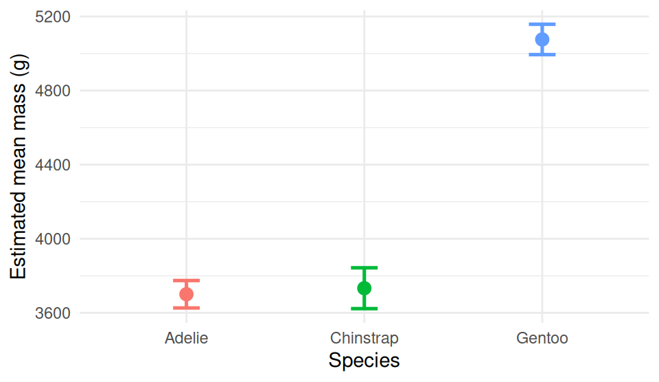

Estimated marginal means with 95% confidence intervals.

• Non-overlapping intervals hint at real differences
• Pair this plot with the letters for a publication-ready figure

The emmeans plot is the ANOVA cousin of Lecture 03’s mean ± SE plot.

How to Report an ANOVA

# Pull the F table values for reporting ---------------
mass_tab <- Anova(mass_model, type = "II")
mass_tab

Anova Table (Type II tests)

Response: body_mass_g
             Sum Sq  Df F value    Pr(>F)    
species   146864214   2  343.63 < 2.2e-16 ***
Residuals  72443483 339                      
---
Signif. codes:  0 '***' 0.001 '**' 0.01 '*' 0.05 '.' 0.1 ' ' 1

“Body mass differed significantly among the three penguin species (one-way ANOVA: F(2, 339) = 343.6, p < 0.001). Tukey-adjusted comparisons showed all three species differed, with Gentoo heaviest and Adelie lightest.”

Always include:

• Test type (one-way ANOVA)
• F, both df, and the p-value
• The post-hoc result (which groups differ)
• Group means ± SE or CI

Never write “p = 0.000” — use “p < 0.001”.

🛑 Pause — Do Activity Parts 9–11 Now

Run the emmeans pairwise test, get the letters, plot the means ± CI, and write your results sentence. Predict which species differ before you run the comparisons.

What We Learned Today

Concepts:

• ANOVA rejects H₀ for the group, but post-hoc finds which pairs differ
• Tukey adjustment keeps the family-wise error at 0.05
• A compact letter display turns a pairwise table into one glance

R skills:

• aov() + summary()
• car::Anova(model, type = "II")
• emmeans(model, pairwise ~ group) + multcomp::cld()

References:

• 📖 W&S Ch. 15 — ANOVA
• 📖 emmeans vignettes

Up next — Lecture 15:

• Kicking off the final project
• Applying this whole toolkit — wrangling, plotting, and a test — to a dataset you choose