Lecture 11 — Linear Regression

Using one measurement to predict another (Whitlock & Schluter Ch. 17)

Fitting a linear regression with lm(), reading the summary() output, checking the residuals, and using predict() to turn a mass into an area.

Where we left off (Lectures 09–10)

• Five steps — hypotheses → check normality → check variance → run the test → interpret and report
• Welch’s t-test compares the means of two groups
• Pseudoreplication — average up to the thing you actually sampled before you test
• Our leaves — mean leaf mass did not differ between the shady and sunny sides
• Our sugar maples — shady-side leaves were significantly larger in area than sunny-side leaves on the same tree

Note

✅ Where today comes in

• A t-test compares two groups.
• Today we ask a different question:
  • can one number predict another number?
  • we weighed our leaf tracings, but what we actually want is leaf area in cm²

Goals for Today

• Understand what a linear regression does: fit a straight line, \(\hat{Y} = a + bX\)
• See what a residual is, in a real plot
• Fit a model with lm()
• Read and interpret the summary() output — slope, p-value, R²
• Check the residuals the way R shows them to you
• Use predict() to turn a tracing mass into a leaf area
• Report the result in a standard sentence

• Tools today:
  • lm() — fit the line
  • summary() — read the result
  • plot(model) — check the residuals
  • predict() — make predictions
  • geom_smooth(method = "lm") — draw the line
• Reading:
  • 📖 Whitlock & Schluter, Ch. 17 — Regression
    • §17.1 Linear regression
    • §17.3 Testing the slope
    • §17.4 R²
    • §17.5 Assumptions
• Today’s naming:
  • models → _model
  • plots → _plot

🧩 Chunk 1 of 3 · What Regression Does

• We will cover:

• the question regression answers,

• the equation \(\hat{Y} = a + bX\),

• what a residual is,

• what R² tells you,

• and the assumptions.

• No code in this chunk — just the idea.

What Is Linear Regression?

Linear regression fits the best straight line through a cloud of points so you can predict one number (Y) from another number (X).

Role	Variable	On the plot
Explanatory (X)	what you can measure easily	x-axis
Response (Y)	what you actually want to know	y-axis

X is usually the easy measurement. Y is the expensive one. Regression gives you an equation that converts X into Y.

📖 W&S §17.1 p. 540–541

Regression vs. the t-test:

Test	The question
t-test	Do two groups have different means?
Regression	Does X predict Y?

Use regression when:

• both variables are numeric
• X could reasonably predict Y
• you want an equation, not just a yes/no

A Real Example from the Textbook

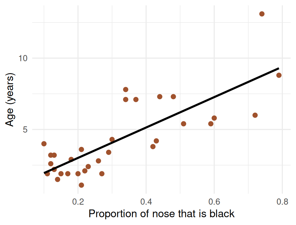
W&S Example 17.1 — “the lion’s nose.” 32 male lions of known age.

Aging a wild lion is hard — you have to have watched it since it was a cub.

But a male lion’s nose darkens as it ages, and you can photograph a nose from a truck.

• X = proportion of the nose that is black — easy
• Y = age in years — what you want

Fit the line once on lions of known age, and from then on you can estimate a lion’s age from a photograph.

📖 W&S §17.1, Example 17.1

Our Version of the Same Problem

The problem: we want leaf area in cm², but we don’t have a leaf-area meter. We have a balance.

The fix — a calibration curve:

1. Cut paper squares of known area (1, 4, 16 … 567 cm²)
2. Weigh each square
3. Fit the line: area ~ mass
4. Trace a leaf onto the same paper and weigh the tracing
5. Put the tracing mass into the equation → predicted leaf area

Why it works: paper from one stock has a constant area per gram, so mass and area move together almost perfectly.

Known area (cm²)	Squares weighed
1	25
4	32
16	24
36	3
64	7
100	14
225–567	13

118 paper squares in all.

Remember paper_mass_g in our leaf data? That is the tracing mass. By the end of today it becomes an area.

The Regression Equation

\[\hat{Y} = a + bX\]

Symbol	Name	What it means
\(\hat{Y}\)	predicted Y	what the line says Y should be
a	intercept	Y when X = 0 — where the line crosses
b	slope	how much Y changes per 1 unit of X

Ours will read:

\[\widehat{\text{area}} = a + b \times \text{mass}\]

📖 W&S §17.1 pp. 543–545

The slope is the useful one.

b = the extra cm² you get for each extra gram of paper

That is just the area density of the paper stock — and it is the number that does the converting.

The intercept is a bookkeeping number.

a = the predicted area of a piece of paper weighing nothing

Physically that should be 0. A small value near zero is fine; it is measurement noise, not biology.

What Is a Residual?

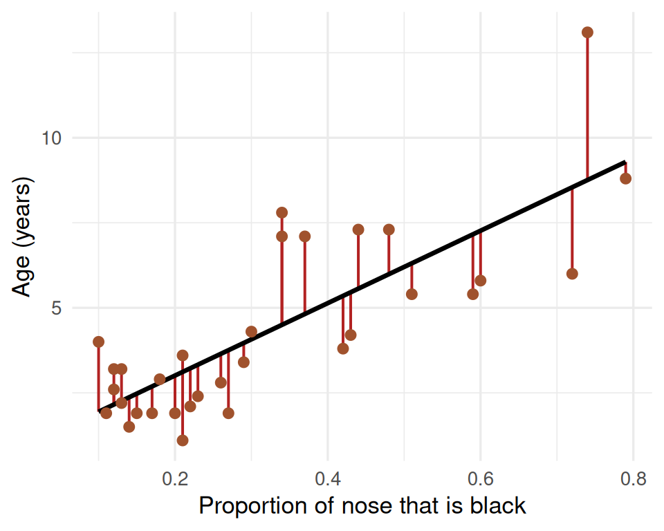
Red = the residuals for the lion data.

A residual is one point’s miss:

\[\text{residual} = \text{observed} - \text{predicted}\]

• A point above the line → positive residual (that lion was older than its nose suggested)
• A point below the line → negative residual
• A point on the line → residual of 0

The line R gives you is the one that makes those red segments as small as possible overall. That is all “least squares” means — and R does the work.

📖 W&S §17.1 p. 542

R² — How Tight Is the Fit?

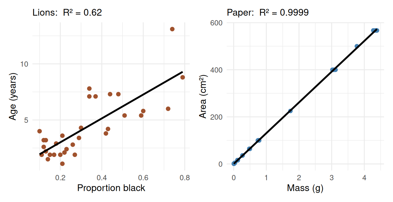
R² runs from 0 to 1. It is the fraction of the variation in Y that the line accounts for.

R²	Reads as
1.00	points sit on the line
0.62	X explains 62% of the variation
0.00	the line tells you nothing

Both of these are good regressions. Nose blackness really does predict a lion’s age — just with scatter, because lions vary. Paper is manufactured to be uniform, so it has almost none.

In biology, R² of 0.3–0.7 is normal and useful. Don’t expect 0.99.

📖 W&S §17.4 p. 555

R² and the p-value Answer Different Questions

	The question it answers
p-value	Is there really a relationship, or could this slope be chance?
R²	How tightly do the points follow the line?

You can have a significant slope with a low R² — a real relationship with a lot of scatter. That is most of ecology.

Important

The slope is the hypothesis test.

H₀: the slope is 0 — X does not predict Y

Hₐ: the slope is not 0 — X does predict Y

summary() gives you the p-value for exactly that test, and we will find it on the next few slides.

📖 W&S §17.3 pp. 551–553

Assumptions of Regression

Four things need to be roughly true for the p-value and the intervals to mean anything (W&S §17.5):

#	Assumption	How you check it
1	Linear — Y really does follow a straight line	the scatter plot, then plot(model) panel 1
2	Independent — one observation doesn’t depend on another	your study design
3	Equal variance — the scatter is about the same all the way along	plot(model) panels 1 and 3
4	Normal residuals — the misses are bell-shaped	plot(model) panel 2

Important

Check the residuals, not the raw data.

Normality here is about the misses — the red segments — not about Y itself. Y is supposed to go up with X; of course it isn’t bell-shaped.

The good news: once you have a fitted model, plot() draws all of these for you. No extra code.

Same habit as the t-test: check → decide → report.

📖 W&S §17.5 pp. 557–560

🧩 Chunk 2 of 3 · Fit It and Read It

We will cover: loading the paper data, the scatter plot, fitting with lm(), and reading the summary() output line by line.

🛑 After this chunk: Activity Parts 1–4 (load, plot, fit, read the summary).

Load Libraries and Data

# Load packages at the top ------------------------------
library(readxl)    # read Excel files
library(tidyverse) # dplyr + ggplot2
library(janitor)   # clean_names()

# Load the paper calibration data ----------------------
paper_df <- read_excel("data/paper_area_weights.xlsx")

Two columns, 118 rows: area_cm2 is the known area of each square, mass_g is what it weighed.

Always Plot It First

# Scatter plot of area against mass --------------------
scatter_plot <- paper_df %>%
  ggplot(aes(x = mass_g, y = area_cm2)) +
  geom_point() +
  geom_smooth(method="lm")
scatter_plot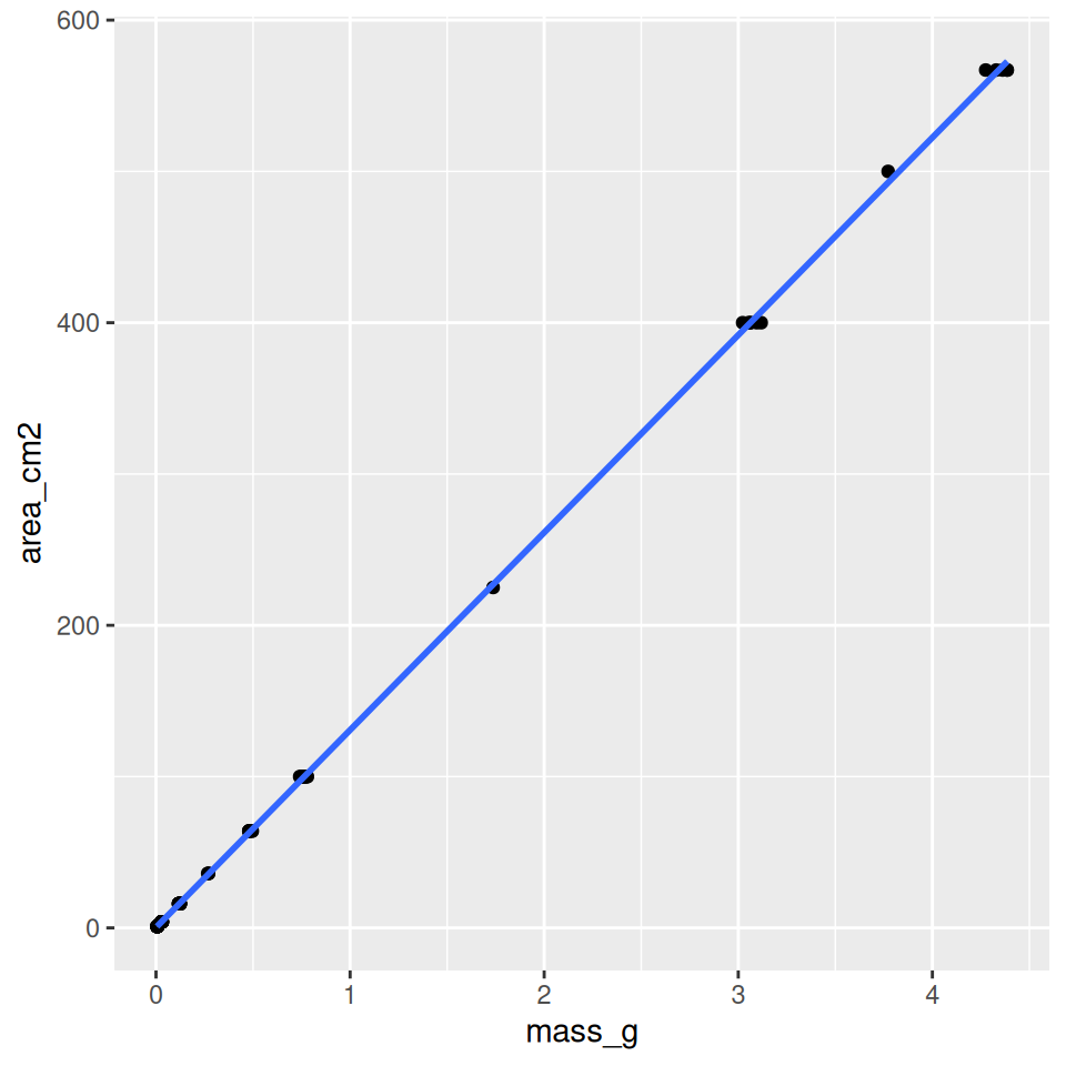

Three plain lines. aes(x = , y = ) puts the explanatory variable on x and the response on y, and geom_point() draws the dots.

What you are looking for:

• Straight? → a line is the right tool
• Scatter the same all the way along?
• Any point way off on its own?

Here: straight, tight, nothing strange. Fit the line.

Note

Never fit a regression you haven’t looked at. A curve, a funnel, or one wild point all change what you should do next.

Fit the Model with lm()

# Fit the regression line ------------------------------
paper_lm_model <- lm(area_cm2 ~ mass_g,
                     data = paper_df)

Nothing prints. lm() hands back a model object that is holding the answer — summary() is what shows it to you.

The formula is the whole trick:

lm(Y ~ X, data = df)

• Y — the response — goes on the left of ~
• X — the explanatory variable — goes on the right
• ~ reads as “is predicted by”

So area_cm2 ~ mass_g is “area is predicted by mass.”

Warning

⚠️ Get the order wrong and R will still answer. lm(mass_g ~ area_cm2) runs fine — it just fits the question you didn’t ask.

summary() — the Whole Output

# Read the model ---------------------------------------
summary(paper_lm_model)

Call:
lm(formula = area_cm2 ~ mass_g, data = paper_df)

Residuals:
    Min      1Q  Median      3Q     Max 
-7.2774 -0.3059 -0.1221  0.2264  8.7592 

Coefficients:
            Estimate Std. Error t value Pr(>|t|)    
(Intercept)   0.2792     0.1812   1.541    0.126    
mass_g      130.5234     0.1473 885.964   <2e-16 ***
---
Signif. codes:  0 '***' 0.001 '**' 0.01 '*' 0.05 '.' 0.1 ' ' 1

Residual standard error: 1.764 on 116 degrees of freedom
Multiple R-squared:  0.9999,    Adjusted R-squared:  0.9999 
F-statistic: 7.849e+05 on 1 and 116 DF,  p-value: < 2.2e-16

There are only four numbers in here that you need, and we will take them one at a time:

1. the slope (mass_g → Estimate)
2. the intercept ((Intercept) → Estimate)
3. the slope’s p-value (mass_g → Pr(>|t|))
4. the R² (Multiple R-squared)

Reading It — 1. The Coefficients Table

Coefficients:
            Estimate Std. Error t value Pr(>|t|)
(Intercept)   0.2792     0.1812   1.541    0.126
mass_g      130.5234     0.1473 885.964   <2e-16

The Estimate column is the equation.

• (Intercept) = 0.28 → that is a
• mass_g = 130.52 → that is b, the slope

So the fitted line is:

\[\widehat{\text{area}} = 0.28 + 130.52 \times \text{mass}\]

Say the slope out loud, with units:

Every extra 1 gram of this paper is another 130.5 cm² of area.

That is the conversion factor we came for.

The other three columns, in one line each:

Column	What it is
Std. Error	how uncertain that estimate is
t value	Estimate ÷ Std. Error
Pr(>|t|)	the p-value for that row

📖 W&S §17.3 p. 551

Reading It — 2. The Two p-Values

(Intercept)   0.2792   ...   0.126
mass_g      130.5234   ...  <2e-16

The slope row is the one that matters. Pr(>|t|) for mass_g is <2e-16 — R’s way of writing “smaller than I can print.”

• H₀: the slope is 0 → mass tells you nothing about area
• p < 0.001 → reject H₀. Mass predicts area.

The intercept row: p = 0.126, so the intercept is not distinguishable from 0 — exactly what physics says it should be. A piece of paper with no mass has no area.

Tip

Which p-value do I report?

The slope’s. That is the biological question. Nobody reports the intercept’s p-value unless zero means something special.

Note

Never write p = 0. When R prints <2e-16, you write p < 0.001.

Reading It — 3. R² and the Bottom Line

Residual standard error: 1.764 on 116 degrees of freedom
Multiple R-squared:  0.9999, Adjusted R-squared:  0.9999
F-statistic: 7.849e+05 on 1 and 116 DF,  p-value: < 2.2e-16

• Multiple R-squared = 0.9999 → mass explains 99.99% of the variation in area. That is manufactured paper, not biology.
• F-statistic with 1 and 116 DF, p < 2.2e-16 → the overall test of the model. With one X it tells you the same thing as the slope’s p-value.
• Residual standard error = 1.76 cm² → a typical miss is about 1.8 cm².

Where the df come from:

• 1 = one explanatory variable
• 116 = 118 squares − 2 numbers we estimated (a and b)

Use Adjusted R-squared once you have more than one X; with a single X, report Multiple R-squared.

Important

R² = 0.9999 does not mean “everything is fine.” It means the points are close to the line. Whether the assumptions hold is a separate question — and we check it two slides from now.

→ ACTIVITY 11 Parts 1–4 now

🛑 Do Activity Parts 1–4 now

Load the paper data, make the scatter plot, fit lm(area_cm2 ~ mass_g), and pull the slope, the p-value, and R² off the summary output — writing them in your answer boxes.

🧩 Chunk 3 of 3 · Plot It, Check It, Use It

We will cover: drawing the fitted line, reading plot(model), using predict() on one tracing and then on a whole column, and writing the result up.

🛑 After this chunk: Activity Parts 5–9 (plot the line, check the residuals, predict, report).

Draw the Line

# Scatter plot with the fitted line --------------------
calibration_plot <- paper_df %>%
  ggplot(aes(x = mass_g, y = area_cm2)) +
  geom_point() +
  geom_smooth(method = "lm")
calibration_plot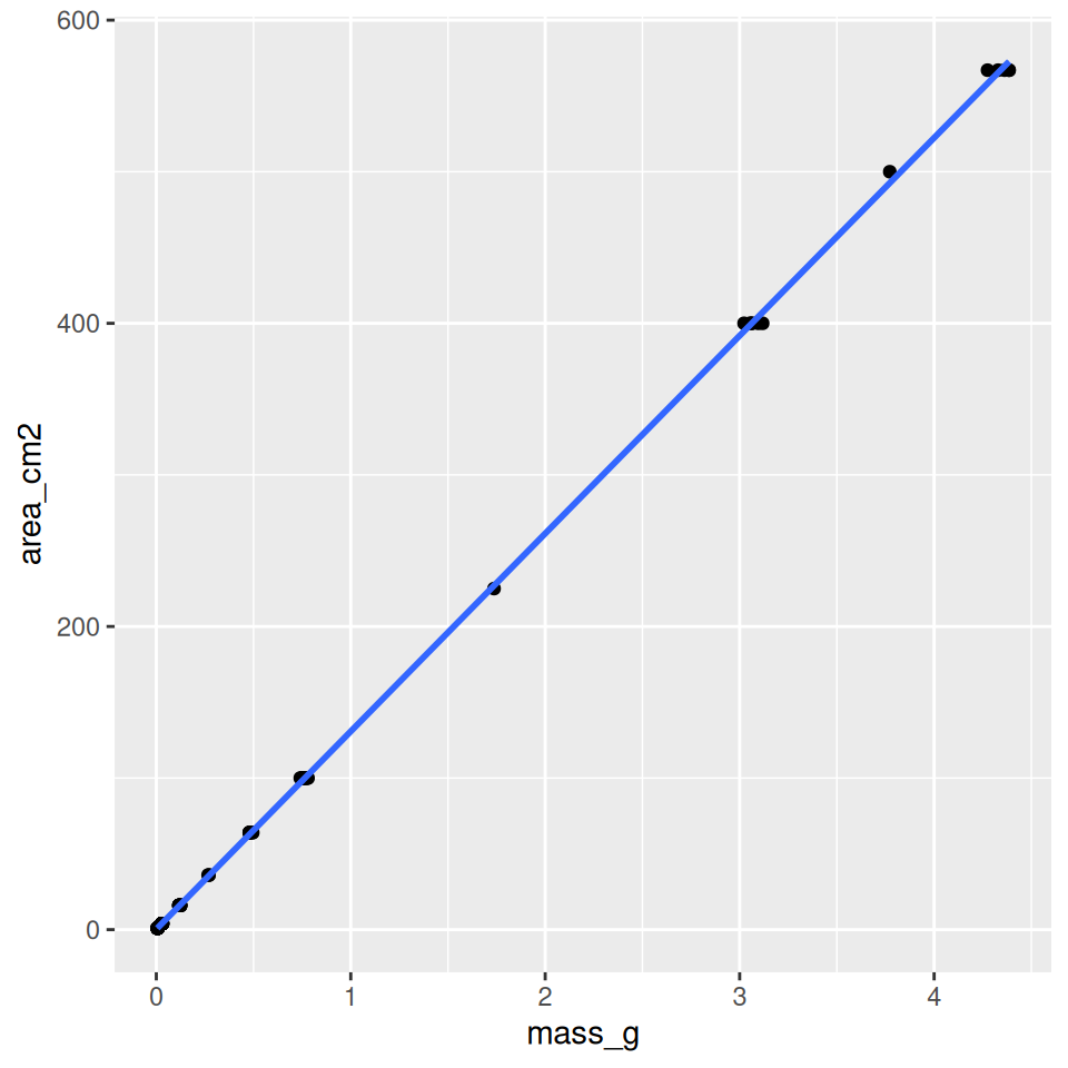

One extra line. geom_smooth(method = "lm") fits the same regression again, just for drawing, and adds:

• the fitted line
• a grey 95% confidence band around it

The band is narrowest in the middle of the data and flares at the ends — the line is pinned down best where you have the most data. Here it is so narrow you can barely see it.

Note

geom_smooth() defaults to a wiggly curve. method = "lm" is what makes it a straight regression line.

The Same Plot, Dressed Up

# The publication version — for reference ---------------
calibration_plot <- paper_df %>%
  ggplot(aes(x = mass_g, y = area_cm2)) +
  geom_point() +
  geom_smooth(method = "lm") +
  labs(x = "Paper mass (g)",
       y = "Paper area (cm²)") +
  theme_minimal()
calibration_plot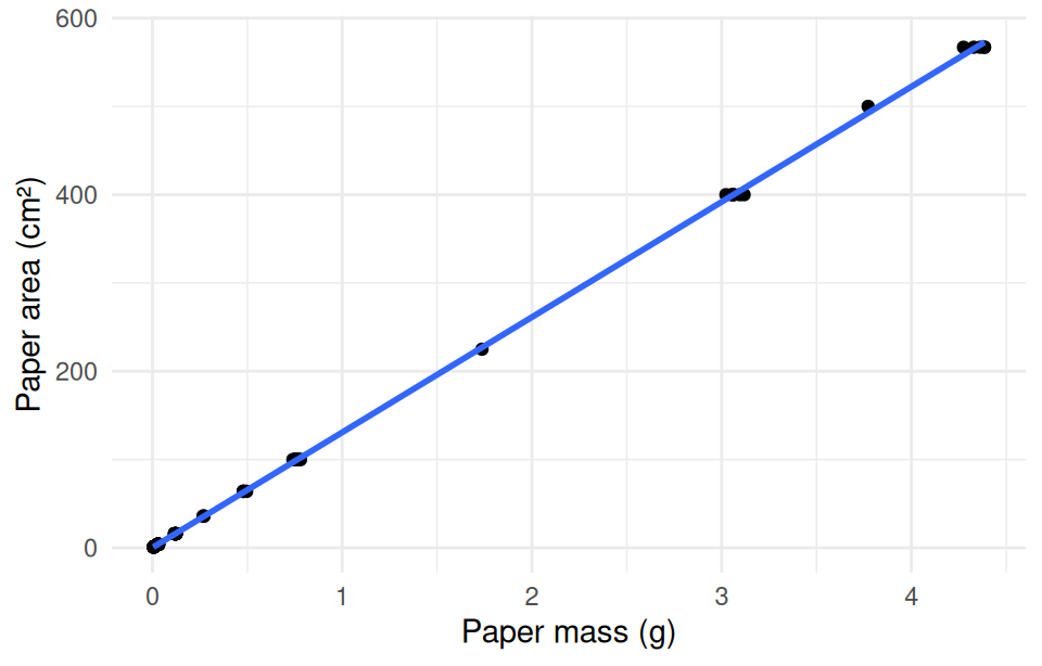

This is the version you’d put in a report — and it is only two additions to the plot you already made:

• labs() — real axis labels with units
• theme_minimal() — drop the grey background

Tip

Don’t type this today. Get the plain geom_point() + geom_smooth(method = "lm") working first. Labels and themes are the last thing you add, once you know the plot is right.

Check the Residuals — plot(model)

# All four residual plots in one call ------------------
par(mfrow = c(2, 2))
plot(paper_lm_model)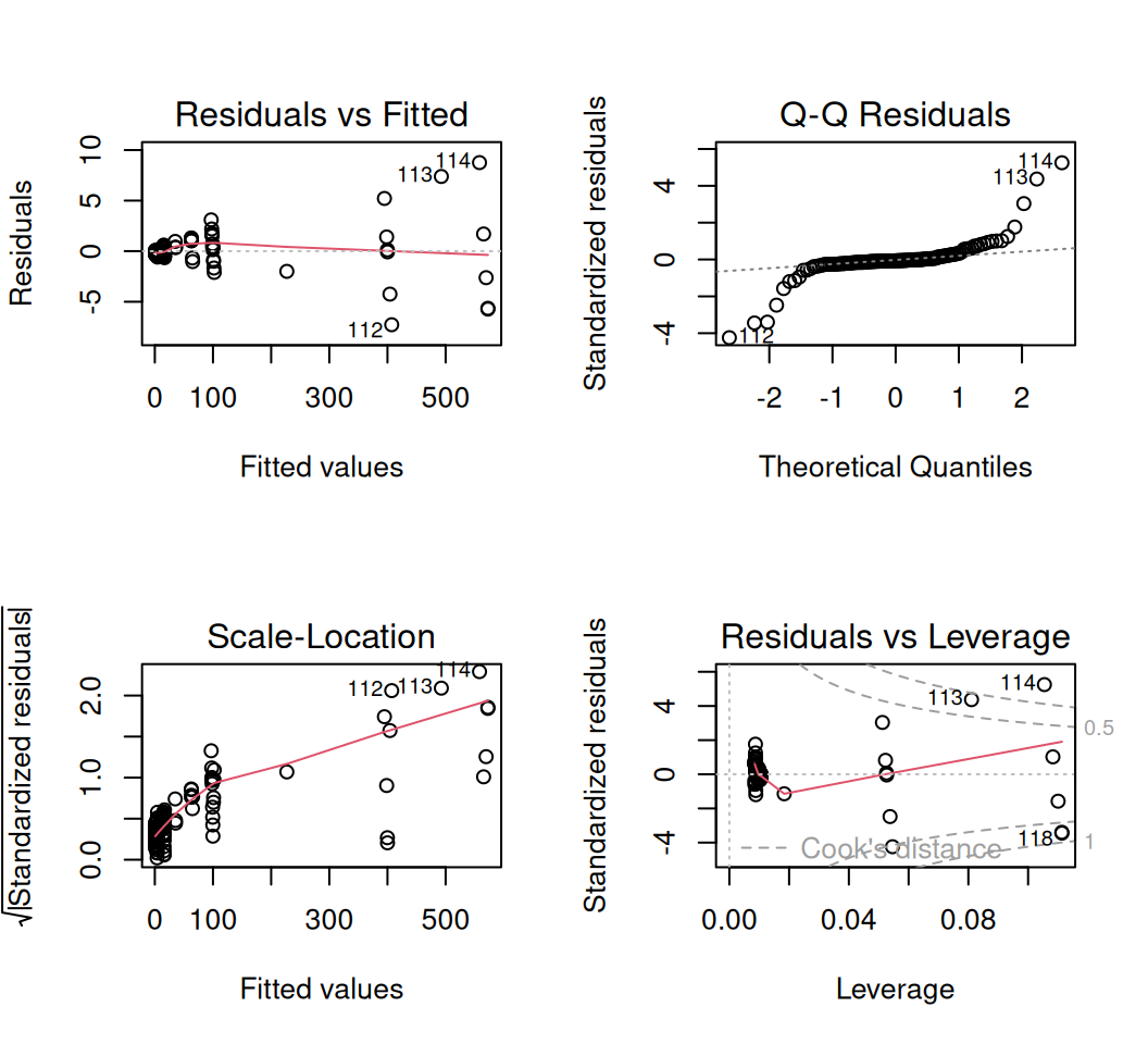

par(mfrow = c(2, 2)) just says “put the next four plots in a 2×2 grid.”

Panel	Name	Checks
1	Residuals vs Fitted	linear? equal scatter?
2	Normal Q-Q	residuals bell-shaped?
3	Scale-Location	equal scatter again
4	Residuals vs Leverage	any one point running the show

Panel 1 is the one to look at first.

• ✅ Good: a flat, shapeless cloud around 0
• ❌ Curved: the relationship isn’t straight
• ❌ Funnel: the scatter grows as Y grows

What Our Residual Plot Is Telling Us

Look at panel 1 again. The points fan out — a 1 cm² square misses by hundredths of a cm², a 567 cm² square misses by several cm².

That is a funnel: assumption 3 (equal variance) does not hold.

# How big are the misses at each square size? ---------
paper_df %>%
  mutate(residual = residuals(paper_lm_model)) %>%
  group_by(area_cm2) %>%
  summarize(biggest_miss = round(max(abs(residual)), 2))

# A tibble: 10 × 2
   area_cm2 biggest_miss
      <dbl>        <dbl>
 1        1         0.35
 2        4         0.59
 3       16         0.65
 4       36         0.96
 5       64         1.3 
 6      100         3.09
 7      225         2   
 8      400         7.28
 9      500         7.39
10      567         8.76

Important

A great R² and a bad residual plot can live together. R² says the points are near the line. The residual plot says the size of the miss depends on how big the square is — which it does, because a balance has percentage error, not fixed error.

So what do we do?

• For predicting a leaf tracing (0.1–0.4 g) we are down in the tight end of the line, where a typical miss is a fraction of a cm². The calibration is fine for the job.
• The confidence intervals at the big-square end are the part you shouldn’t trust.
• The proper fix — fitting on a log scale, or weighting the points — is a graduate topic. Knowing to look, and saying what you saw, is the undergraduate job.

Predict One Tracing

# Predict the area of one leaf tracing ----------------
# The tracing weighed 0.138 g
one_tracing <- tibble(mass_g = 0.138)

predict(paper_lm_model, newdata = one_tracing)

       1 
18.29144 

An 0.138 g tracing is about 18.3 cm² of leaf.

predict() takes two things:

• the model you fitted
• newdata = — a small data frame of the X values you want predictions for

Warning

⚠️ The column in newdata must have the same name as in the model. The model was built on mass_g, so newdata needs a column called mass_g. Call it mass and R stops with “object ‘mass_g’ not found.”

This beats doing the arithmetic yourself — no copying the slope, nothing to mistype.

Predict with an Interval

# Two tracings, with 95% prediction intervals ---------
two_tracings <- tibble(mass_g = c(0.092, 0.138))

predict(paper_lm_model,
        newdata = two_tracings,
        interval = "prediction")

       fit       lwr      upr
1 12.28736  8.777018 15.79771
2 18.29144 14.781578 21.80131

The 0.138 g tracing is 18.3 cm², somewhere between about 14.8 and 21.8 cm².

interval = "prediction" adds two columns:

• fit — the prediction
• lwr and upr — the 95% range

Two kinds of interval:

interval =	Range for	Width
"confidence"	the average area of all tracings this heavy	narrower
"prediction"	one particular tracing	wider

For a single real leaf, use "prediction".

📖 W&S §17.2 pp. 548–550

Convert a Whole Column of Tracings

# Load our leaf data ----------------------------------
leaf_df <-
  read_excel("data/2026_09_03_data_sci_leaf_area.xlsx") %>%
  clean_names()

# Turn every tracing mass into an area ----------------
leaf_df <- leaf_df %>%
  mutate(leaf_area_cm2 =
           predict(paper_lm_model,
                   newdata = tibble(mass_g = paper_mass_g)))

leaf_df %>%
  select(teams, shade, mass_g, paper_mass_g, leaf_area_cm2)

# A tibble: 53 × 5
   teams shade mass_g paper_mass_g leaf_area_cm2
   <chr> <chr>  <dbl>        <dbl>         <dbl>
 1 12345 sunny   0.4          0.21          27.7
 2 12345 sunny   0.48         0.21          27.7
 3 12345 sunny   0.34         0.21          27.7
 4 12345 sunny   0.65         0.24          31.6
 5 12345 sunny   0.27         0.15          19.9
 6 12345 sunny   0.43         0.34          44.7
 7 12345 shady   0.39         0.29          38.1
 8 12345 shady   0.45         0.25          32.9
 9 12345 shady   0.6          0.23          30.3
10 12345 shady   0.57         0.28          36.8
# ℹ 43 more rows

This is the payoff. paper_mass_g was the mass of each leaf’s tracing. Now every leaf has a leaf_area_cm2.

The one fiddly bit is the same rule as before: predict() wants a column called mass_g, so we hand it tibble(mass_g = paper_mass_g) — our tracing masses, under the name the model knows.

Note

The NAs are honest. One team never weighed their tracings, so those leaves have no area. predict() passes the missing value straight through instead of inventing a number.

Was the Area Different Between Sides?

# Predicted leaf area by side -------------------------
leaf_area_plot <- leaf_df %>%
  ggplot(aes(x = shade, y = leaf_area_cm2)) +
  geom_boxplot() +
  geom_jitter(width = 0.15)
leaf_area_plot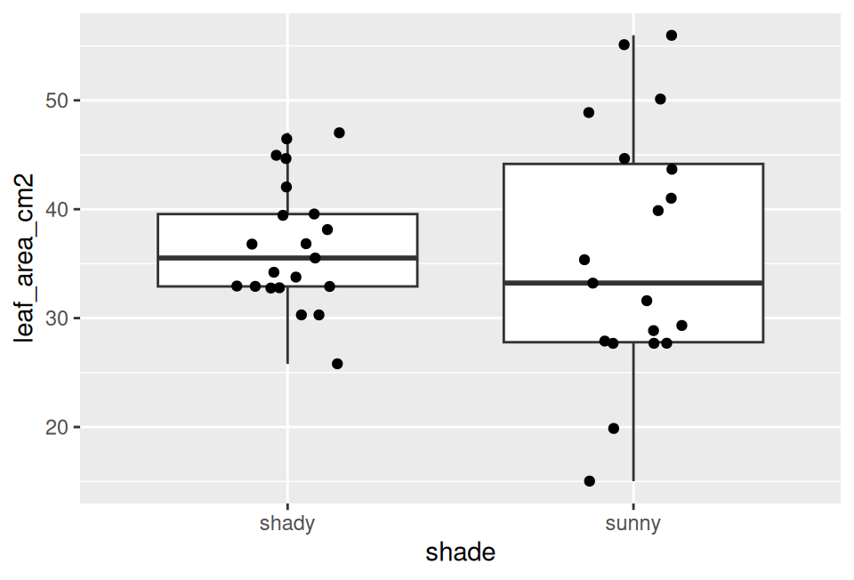

# Mean predicted area per side ------------------------
leaf_df %>%
  group_by(shade) %>%
  summarize(
    n = sum(!is.na(leaf_area_cm2)),
    mean_area = mean(leaf_area_cm2, na.rm = TRUE)
  )

# A tibble: 2 × 3
  shade     n mean_area
  <chr> <int>     <dbl>
1 shady    21      36.7
2 sunny    19      36.0

About 37 cm² on the shady side and 36 cm² on the sunny side — the same story the t-test told us about mass, now in the units we actually wanted.

Note

✅ Why this matters. “Shady leaves weigh 0.02 g more” means little to a reader. “Shady leaves are about 1 cm² bigger” is a sentence an ecologist can use.

How to Report a Regression

The template — fill in from your summary() output:

[What predicted what] (linear regression: F(df₁, df₂) = ___, p ___, R² = ___). The fitted equation was Y = ___ + ___ × X.

Ours:

Paper mass was a very strong predictor of paper area (linear regression: F(1, 116) = 784,900, p < 0.001, R² = 0.9999). The calibration equation was area = 0.28 + 130.52 × mass. Residual scatter increased with square size, so intervals for the largest squares should be treated with caution.

Where every number comes from:

In the sentence	In summary()
F and both df	the F-statistic: line
p	that same line
R²	Multiple R-squared
intercept	(Intercept) → Estimate
slope	mass_g → Estimate

Always include: the test name, F with both df, p, R², and the equation. Add a line about the assumptions you checked.

📖 W&S §17.3 p. 553

→ ACTIVITY 11 Parts 5–9 now

🛑 Do Activity Parts 5–9 now

• Draw the line and run plot(model)
• Predict one tracing, then convert the whole paper_mass_g column into areas
• Write your results sentence
• Your answers in the script are what you hand in

What We Learned Today

The ideas:

• Regression fits a line so you can predict Y from X
• \(\hat{Y} = a + bX\) — the slope converts X into Y
• A residual is one point’s miss: observed − predicted
• R² = how tight the fit is; p = whether the slope is real
• Check the residuals — and say what you saw

The code:

• lm(Y ~ X, data = df) — fit it
• summary(model) — slope, intercept, p, R²
• geom_smooth(method = "lm") — draw it
• plot(model) — check it
• predict(model, newdata = ...) — use it

• Hand in: your finished scripts/11_regression.R — the code is given; your answers are graded

📖 W&S Ch. 17:

• §17.1 Linear regression · §17.2 Prediction
• §17.3 Testing the slope · §17.4 R²
• §17.5 Assumptions

Up next — Lecture 12:

• Pulling real climate data into R with GSODR
• Summarizing daily weather into yearly values
• The same lm() — temperature predicted by date
  • the slope becomes a rate of change per year
  • and you write that regression yourself