Lecture 10 — Factors: Taming Categorical Data

Ordering, renaming, and lumping categories with forcats — and cleaner ggplots

factors

forcats

tidyverse

ggplot

Categorical variables are factors, and factors carry an ORDER. This 2-day lecture shows how to create and inspect factors, reorder them for readable ggplots (fct_reorder, fct_infreq), rename/collapse/lump levels, set the reference group for an ANOVA (fct_relevel), and avoid the classic factor traps — all using the Palmer penguins data.

Author

Bill Perry

Published

July 5, 2026

Where we left off — Pivoting real data

pivot_longer() / pivot_wider() — reshaped the messy Lake Superior ice data
group_by() + summarize() and lm() on the tidied result
But every plot still put categories in alphabetical order

Note

✅ Transition

Why alphabetical? Because a categorical column is a factor, and its levels default to alphabetical. Today we take control of that order — and of the labels — with the forcats package. You’ll lean on it again next week when you run a one-way ANOVA.

Goals for today (a 2-day lecture)

What a factor is and why R uses them
Create & inspect — factor(), levels(), fct_count()
Reorder for plots — fct_reorder(), fct_infreq(), fct_rev()
Rename & simplify — fct_recode(), fct_collapse(), fct_lump()
Set a model’s reference level — fct_relevel()
Drop unused levels and dodge the classic traps

Tools today:

tidyverse (includes forcats)
palmerpenguins

Textbook:

📖 R4DS Ch. 16 — Factors
📖 R4DS Ch. 9 — Layers

Tip

Day 1: create, inspect, reorder. Day 2: rename, lump, model.

How to Use These Slides — Predict · Type · Run

This lecture runs in four short chunks over two days. After each chunk you switch to the activity and type the code yourself.

For every code block, do three things:

Predict — before it runs, say what the plot or output will look like
Type it out by hand — do not copy-paste
Run it and compare to your prediction

Note

✅ Why bother? (the evidence)

Predicting the order of a plot forces you to reason about levels — the whole point of factors.
Typing by hand builds the muscle memory for the fct_ family.
Chunk → practice keeps each idea in working memory long enough to stick.

🧩 Chunk 1 of 4 · What a Factor Is (Day 1)

We will cover: what factors are, why alphabetical order is a problem, and how to create and inspect them.

Tip

🖐 After this chunk: Activity Parts 1–3 (inspect the penguin factors).

What Is a Factor?

A factor is a categorical variable with a fixed, known set of values — its levels — stored in a specific order.

Under the hood: integer codes (1, 2, 3…) plus a labels table
The order of the levels controls plot axes, legends, and model baselines
Different from a plain character string, which has no built-in order

Note

📖 New word

forcats = “for categorical variables” — the tidyverse package (loaded with library(tidyverse)) for working with factors. Every function starts with fct_.

The Problem Factors Solve — Alphabetical Order

Note

🔮 Predict first: If we make a bar chart of penguin species with no other instructions, in what order will the three bars appear?

# Load packages + data --------------------------------
library(tidyverse)      # includes forcats
library(palmerpenguins)

# Swap this one line to use your own data later -------
penguins_df <- penguins %>% drop_na(species, body_mass_g)

# ggplot uses the factor's level order = ALPHABETICAL -
penguins_df %>%
  ggplot(aes(x = species)) +
  geom_bar() +
  theme_minimal()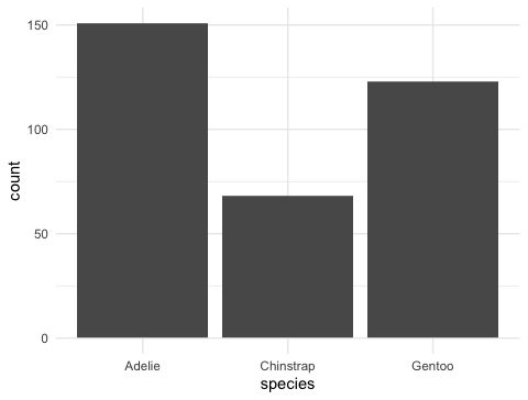

Adelie, Chinstrap, Gentoo — alphabetical, because that is the default level order.

Alphabetical is almost never the order you want to show. Factors let you fix that in one line.

📖 R4DS §16.5 — modifying factor order

Create & Inspect Factors

# What type is species, and what are its levels? ------
class(penguins_df$species)

[1] "factor"

levels(penguins_df$species)

[1] "Adelie"    "Chinstrap" "Gentoo"

# fct_count() = a factor-aware count -------------------
fct_count(penguins_df$species)

# A tibble: 3 × 2
  f             n
  <fct>     <int>
1 Adelie      151
2 Chinstrap    68
3 Gentoo      123

class() — confirms it’s a factor
levels() — the ordered set of categories
fct_count() — how many rows per level (even levels with zero rows show up!)

Tip

Make a factor from a string with factor(x) or as_factor(x).

🛑 Pause — Do Activity Parts 1–3 Now

Load the penguins, confirm species and island are factors, list their levels, and make the default (alphabetical) bar chart. Predict the order before you run it.

🧩 Chunk 2 of 4 · Reorder for Readable Plots (Day 1)

We will cover: the payoff — reordering factor levels so plots tell the story, with fct_infreq(), fct_reorder(), and fct_rev().

Tip

🖐 After this chunk: Activity Parts 4–6 (reorder bars and boxplots).

`fct_infreq()` — Order by Frequency

# Order bars from most to least common ----------------
penguins_df %>%
  mutate(species = fct_infreq(species)) %>%
  ggplot(aes(x = species)) +
  geom_bar() +
  theme_minimal()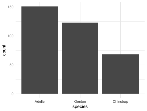

fct_infreq() — biggest group first
Add fct_rev() to flip to smallest-first
Perfect for bar charts of counts — the reader sees the ranking instantly

Note

You reorder inside mutate(), then plot. The data itself is unchanged elsewhere.

`fct_reorder()` — Order by Another Variable

Note

🔮 Predict first: We’ll reorder species by their median body mass. Which species ends up last (heaviest)?

# Order species by MEDIAN body mass, low -> high ------
penguins_df %>%
  mutate(species = fct_reorder(species, body_mass_g, .fun = median)) %>%
  ggplot(aes(x = species, y = body_mass_g, fill = species)) +
  geom_boxplot(alpha = 0.6) +
  theme_minimal() +
  theme(legend.position = "none")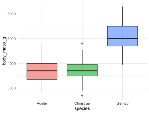

This is the one you’ll use constantly.

fct_reorder(f, x, .fun) — order the factor f by a summary of x
Boxplots, dot plots, lollipop charts all read better ordered by value, not alphabet

📖 R4DS §16.4 — fct_reorder()

`fct_rev()` and Ordered Summary Plots

# Mean mass per species, ordered high -> low ----------
penguins_df %>%
  group_by(species) %>%
  summarize(mean_mass = mean(body_mass_g)) %>%
  mutate(species = fct_reorder(species, mean_mass) %>% fct_rev()) %>%
  ggplot(aes(x = mean_mass, y = species)) +
  geom_col(fill = "steelblue") +
  labs(x = "Mean mass (g)", y = NULL) +
  theme_minimal()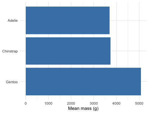

fct_rev() — reverse the current order
Horizontal bars ordered by value = the cleanest ranking plot there is
Chaining fct_reorder() %>% fct_rev() puts the biggest bar on top

🛑 End of Day 1 · Start Day 2 Here

Day 1 recap — you can now:

Say what a factor is and why level order matters
Inspect levels with levels() and fct_count()
Reorder for plots with fct_infreq(), fct_reorder(), fct_rev()

Day 2 — the deeper cuts:

Rename, collapse, and lump levels
Set the reference group for a model
Drop ghost levels, and dodge the classic traps

🧩 Chunk 3 of 4 · Rename, Collapse, Lump (Day 2)

We will cover: cleaning up messy level labels — fct_recode(), fct_collapse(), fct_lump().

Tip

🖐 After this chunk: Activity Parts 7–9 (rename and lump levels).

`fct_recode()` — Rename Levels

# Give levels cleaner display names -------------------
penguins_df %>%
  mutate(species = fct_recode(species,
    "Adélie penguin"    = "Adelie",
    "Chinstrap penguin" = "Chinstrap",
    "Gentoo penguin"    = "Gentoo"
  )) %>%
  count(species)

# A tibble: 3 × 2
  species               n
  <fct>             <int>
1 Adélie penguin      151
2 Chinstrap penguin    68
3 Gentoo penguin      123

fct_recode(f, "new" = "old", ...) — rename one or more levels
New name on the left, old on the right
Great for turning codes or abbreviations into report-ready labels

Warning

⚠️ Watch out! A misspelled old name is silently ignored — check your levels after.

`fct_collapse()` — Merge Levels into Groups

# Combine several levels into one ---------------------
penguins_df %>%
  mutate(size_group = fct_collapse(species,
    "smaller" = c("Adelie", "Chinstrap"),
    "larger"  = "Gentoo"
  )) %>%
  count(size_group)

# A tibble: 2 × 2
  size_group     n
  <fct>      <int>
1 smaller      219
2 larger       123

fct_collapse() — map many old levels onto a few new ones
Useful for turning fine categories into the groups your question needs
The reverse of splitting — you’re coarsening the variable

`fct_lump()` — Bundle Rare Levels into “Other”

# Keep the 2 most common islands, lump the rest -------
penguins %>%
  drop_na(island) %>%
  mutate(island = fct_lump_n(island, n = 2)) %>%
  count(island)

# A tibble: 3 × 2
  island     n
  <fct>  <int>
1 Biscoe   168
2 Dream    124
3 Other     52

fct_lump_n(f, n) — keep the top n, everything else → “Other”
fct_lump_min(f, min) — lump any level with fewer than min rows
Essential when a variable has a long tail of rare categories

📖 R4DS §16.6 — lumping

Live Demo — Watch It Break (quietly)

Factors look like their labels, but underneath they’re integer codes. So this quietly gives the wrong answer:

years <- factor(c("2010", "2011", "2012"))
as.numeric(years)
#> [1] 1 2 3      # the level CODES, not the years!

The fix — go through character first:

as.numeric(as.character(years))
#> [1] 2010 2011 2012

Important

✅ Why show a quiet break?

No error, just wrong numbers. as.numeric() on a factor returns the 1, 2, 3 level codes, not the labels. Any time a factor holds numbers you need to compute with, convert to character first.

🛑 Pause — Do Activity Parts 7–9 Now

Rename the species to full names, collapse them into size groups, lump the islands, and try the as.numeric() trap yourself. Predict each output before you run it.

🧩 Chunk 4 of 4 · Factors in Models & Cleanup (Day 2)

We will cover: how level order sets the model baseline (fct_relevel), dropping unused levels, and one clean final figure.

Tip

🖐 After this chunk: Activity Parts 10–12 (relevel a model, drop levels, build the final plot).

`fct_relevel()` — Set the Reference Level

Note

🔮 Predict first: When you fit a model — the regression from Lecture 06, or the ANOVA coming next week — R compares everything to the first level (Adelie here). If we make Gentoo the reference, what changes — the overall test, or the coefficients?

# Default reference = Adelie (alphabetical first) -----
coef(lm(body_mass_g ~ species, data = penguins_df))

     (Intercept) speciesChinstrap    speciesGentoo 
      3700.66225         32.42598       1375.35401

# Make Gentoo the reference group ---------------------
penguins_relevel <- penguins_df %>%
  mutate(species = fct_relevel(species, "Gentoo"))

coef(lm(body_mass_g ~ species, data = penguins_relevel))

     (Intercept)    speciesAdelie speciesChinstrap 
        5076.016        -1375.354        -1342.928

fct_relevel(f, "x") — move level x to the front (the reference)
The (Intercept) becomes that group’s mean; other coefficients are differences from it
The overall F-test and p-value don’t change — only the baseline you compare to

📖 R4DS §16.5

Drop Unused Levels After Filtering

# Filter out Gentoo... but the level lingers ----------
two_species <- penguins_df %>% filter(species != "Gentoo")
levels(two_species$species)     # Gentoo is STILL a level!

[1] "Adelie"    "Chinstrap" "Gentoo"

# Remove empty levels ---------------------------------
two_species <- two_species %>% mutate(species = fct_drop(species))
levels(two_species$species)

[1] "Adelie"    "Chinstrap"

filter() removes rows, not levels — a “ghost” level remains
Ghost levels leave empty gaps in plots and empty groups in models
fct_drop() (or droplevels()) clears them out

Warning

⚠️ Watch out! An empty factor level is the #1 cause of a stray blank space on a boxplot axis.

Put It All Together — One Clean Figure

# Reordered + relabeled in one pipeline ---------------
penguins_df %>%
  mutate(
    species = fct_recode(species, "Adélie" = "Adelie"),
    species = fct_reorder(species, body_mass_g, .fun = median)
  ) %>%
  ggplot(aes(x = species, y = body_mass_g, fill = species)) +
  geom_boxplot(alpha = 0.6, outlier.shape = NA) +
  geom_point(position = position_jitter(width = 0.15, seed = 42),
             alpha = 0.3, size = 1.4) +
  labs(x = NULL, y = "Body mass (g)") +
  theme_minimal() +
  theme(legend.position = "none")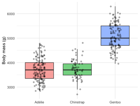

Ordered by mass, relabeled, publication-ready — and the code that made it is three fct_ calls inside one mutate().

This is the everyday payoff: factors are how you make categorical plots say what you mean.

🛑 Pause — Do Activity Parts 10–12 Now

Relevel a model to a new reference, drop an unused level, and build your own reordered + relabeled figure. Predict the reference change before you run it.

What We Learned Today

Concepts:

A factor = categories + a stored order of levels
Level order drives plot axes, legends, and model baselines
Reorder for readable plots: fct_reorder(), fct_infreq(), fct_rev()
Tidy the labels: fct_recode(), fct_collapse(), fct_lump()
Set the model reference with fct_relevel(); clear ghosts with fct_drop()
as.numeric() on a factor returns codes — convert to character first

References:

📖 R4DS Ch. 16 — Factors
📖 common_code/15_factors

Up next — Lecture 11:

One-way ANOVA — compare a numeric response across three or more groups
Your factor levels are now in order, so the group comparisons read cleanly

Other Formats

Where we left off — Pivoting real data

Goals for today (a 2-day lecture)

How to Use These Slides — Predict · Type · Run

🧩 Chunk 1 of 4 · What a Factor Is (Day 1)

What Is a Factor?

The Problem Factors Solve — Alphabetical Order

Create & Inspect Factors

🛑 Pause — Do Activity Parts 1–3 Now

🧩 Chunk 2 of 4 · Reorder for Readable Plots (Day 1)

fct_infreq() — Order by Frequency

fct_reorder() — Order by Another Variable

fct_rev() and Ordered Summary Plots

🛑 End of Day 1 · Start Day 2 Here

🧩 Chunk 3 of 4 · Rename, Collapse, Lump (Day 2)

fct_recode() — Rename Levels

fct_collapse() — Merge Levels into Groups

fct_lump() — Bundle Rare Levels into “Other”

Live Demo — Watch It Break (quietly)

🛑 Pause — Do Activity Parts 7–9 Now

🧩 Chunk 4 of 4 · Factors in Models & Cleanup (Day 2)

fct_relevel() — Set the Reference Level

Drop Unused Levels After Filtering

Put It All Together — One Clean Figure

🛑 Pause — Do Activity Parts 10–12 Now

What We Learned Today

`fct_infreq()` — Order by Frequency

`fct_reorder()` — Order by Another Variable

`fct_rev()` and Ordered Summary Plots

`fct_recode()` — Rename Levels

`fct_collapse()` — Merge Levels into Groups

`fct_lump()` — Bundle Rare Levels into “Other”

`fct_relevel()` — Set the Reference Level