Lecture — One-Way ANOVA I: Setting Up the Test

Why not many t-tests, the F-statistic, ordering groups with factors, fitting the model, and checking assumptions

From two groups to many: why we don’t run many t-tests, how the F-statistic partitions variance, using factors to order groups for a readable plot and to set the ANOVA reference level, fitting a one-way ANOVA as a linear model, and checking its assumptions — normality of residuals and equal variance — on the Palmer penguins data.

Where we left off (Lectures 09–11)

• T-Tests I & II — comparing the means of two groups with Welch’s t-test
• Regression (Lecture 11) — lm(Y ~ X) with a numeric predictor, checked with plot(model)
• Both of those are, underneath, the same tool: a linear model

Note

✅ Transition

The t-test compared two groups. But biology is full of three-or-more group questions — three species, four sites, five treatments. Today’s twist: it’s still lm(Y ~ X) — just with a categorical X instead of a numeric one. That’s one-way ANOVA.

Goals for today

• Understand why we don’t just run many t-tests
• See how the F-statistic compares between- vs within-group variance
• State ANOVA hypotheses (H₀: all means equal)
• Use factors to order groups for a readable plot and set the reference level
• Fit the model with lm()
• Check assumptions — normality of residuals, equal variance

Tools today:

• palmerpenguins, tidyverse (includes forcats)
• car — Levene’s test

Textbook:

• 📖 Whitlock & Schluter, Ch. 15 — ANOVA
• 📖 R4DS Ch. 16 — Factors
• 📖 R4DS Ch. 9 — Layers

Naming: models → _model, plots → _plot

How to Use These Slides — Predict · Type · Run

This lecture runs in two short chunks. After each chunk you switch to the activity and type the code yourself.

For every code block, do three things:

1. Predict — before it runs, say what you think the output will be
2. Type it out by hand — do not copy-paste
3. Run it and compare to your prediction

Note

✅ Why bother? (the evidence)

• With three groups instead of two, it is tempting to just read off which box in the plot looks tallest. Committing to a prediction about the F-statistic before you see it forces you to reason about between- vs. within-group variance instead of eyeballing a boxplot.
• Typing type = "II" yourself in Anova() is what makes you notice it’s there — paste the line and you’ll never ask why it matters for unbalanced groups.
• Practicing each assumption check right after it’s introduced keeps normality-of-residuals and Levene’s test tied to this penguin model instead of turning into two more disconnected rules to memorize.

🧩 Chunk 1 of 2 · Why ANOVA & the F-Statistic

We will cover: why not many t-tests, what ANOVA asks, how F partitions variance, and a first look at the penguin data.

Tip

🖐 After this chunk: Activity Parts 1–3 (load the penguins, explore, state hypotheses).

Why Not Just Run Many t-Tests?

With 3 groups you’d need 3 t-tests (A–B, A–C, B–C). With 4 groups, 6 tests.

Every test at α = 0.05 has a 5% chance of a false positive. Run several and those risks stack up:

• 3 tests → ~14% chance of at least one false positive
• 6 tests → ~26%

ANOVA asks the question once, holding the overall error rate at 0.05.

Important

The multiple-comparisons problem

More tests = more chances to be fooled by noise. ANOVA is the single, honest test for “do any of these groups differ?”

📖 W&S §15.1 — why a single test

What One-Way ANOVA Asks

One numeric response (Y) across the levels of one categorical predictor (X).

	Hypothesis
H₀ — null	all group means are equal (\(\mu_1 = \mu_2 = \mu_3\))
Hₐ — alternate	at least one group mean differs

Note what Hₐ does not say: it does not tell you which group differs — that comes later, from the post-hoc test.

Our question today:

Do the three penguin species differ in body mass?

• Y = body_mass_g
• X = species (Adelie, Chinstrap, Gentoo)

The F-Statistic — Between vs. Within

\[F = \frac{\text{variance BETWEEN groups}}{\text{variance WITHIN groups}}\]

• Between — how far apart the group means are
• Within — how much the individuals scatter inside each group

Big F → the groups are far apart relative to their internal noise → small p-value.

F ≈ 1 → the spread between groups is no bigger than the spread within them → no real difference.

Note

✅ Key idea

ANOVA is a signal-to-noise ratio. The “signal” is the gap between group means; the “noise” is the within-group scatter.

📖 W&S §15.1–15.2

Meet the Data — Palmer Penguins

# Load packages at the top — always -------------------
library(tidyverse)      # wrangling + ggplot2
library(palmerpenguins) # the penguins data
library(car)            # Levene's test, Anova()
library(emmeans)        # post-hoc pairwise tests

# Drop rows missing mass or species -------------------
penguins_df <- penguins %>%
  drop_na(body_mass_g, species)

penguins_df %>% count(species)

# A tibble: 3 × 2
  species       n
  <fct>     <int>
1 Adelie      151
2 Chinstrap    68
3 Gentoo      123

Three species, one lab: body mass (g) of penguins at Palmer Station, Antarctica.

• drop_na() removes rows with missing mass
• count(species) shows the sample size per group

Important

The groups are unbalanced (different n per species) — that matters when we pick our ANOVA type later.

Explore First — Boxplot by Species

Note

🔮 Predict first: Before the plot renders — do you expect all three species to differ, or just one? Which species do you think is heaviest?

mass_box_plot <- penguins_df %>%
  ggplot(aes(x = species, y = body_mass_g, fill = species)) +
  geom_boxplot(alpha = 0.5, outlier.shape = NA) +
  geom_point(
    position = position_jitter(width = 0.15, seed = 42),
    alpha = 0.3, size = 1.5
  ) +
  labs(x = "Species", y = "Body Mass (g)") +
  theme_minimal() +
  theme(legend.position = "none")

mass_box_plot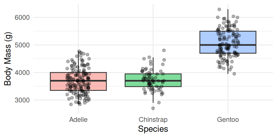

Always plot before you test.

• The picture usually tells the story before the p-value confirms it
• Look for separation between boxes and roughly similar spread
• But notice the order: Adelie, Chinstrap, Gentoo — that’s alphabetical, not by mass

📖 R4DS §9 — Layers

species Is a Factor — and Factors Have an Order

class(penguins_df$species)   # "factor"

[1] "factor"

levels(penguins_df$species)  # the stored order

[1] "Adelie"    "Chinstrap" "Gentoo"   

• A factor is a categorical column with a fixed, ordered set of levels
• ggplot (and lm) draw groups in level order
• The default level order is alphabetical — almost never the order you want

Note

✅ Key idea

Alphabetical order hides the pattern. Ordering the groups by the thing you are testing — here, body mass — makes the boxplot tell the story at a glance.

forcats (the fct_* family) ships with library(tidyverse).

Order the Boxplot by Body Mass — fct_reorder()

penguins_df %>%
  mutate(species = fct_reorder(species, body_mass_g, .fun = median)) %>%
  ggplot(aes(x = species, y = body_mass_g, fill = species)) +
  geom_boxplot(alpha = 0.5, outlier.shape = NA) +
  labs(x = "Species (ordered by median mass)", y = "Body Mass (g)") +
  theme_minimal() +
  theme(legend.position = "none")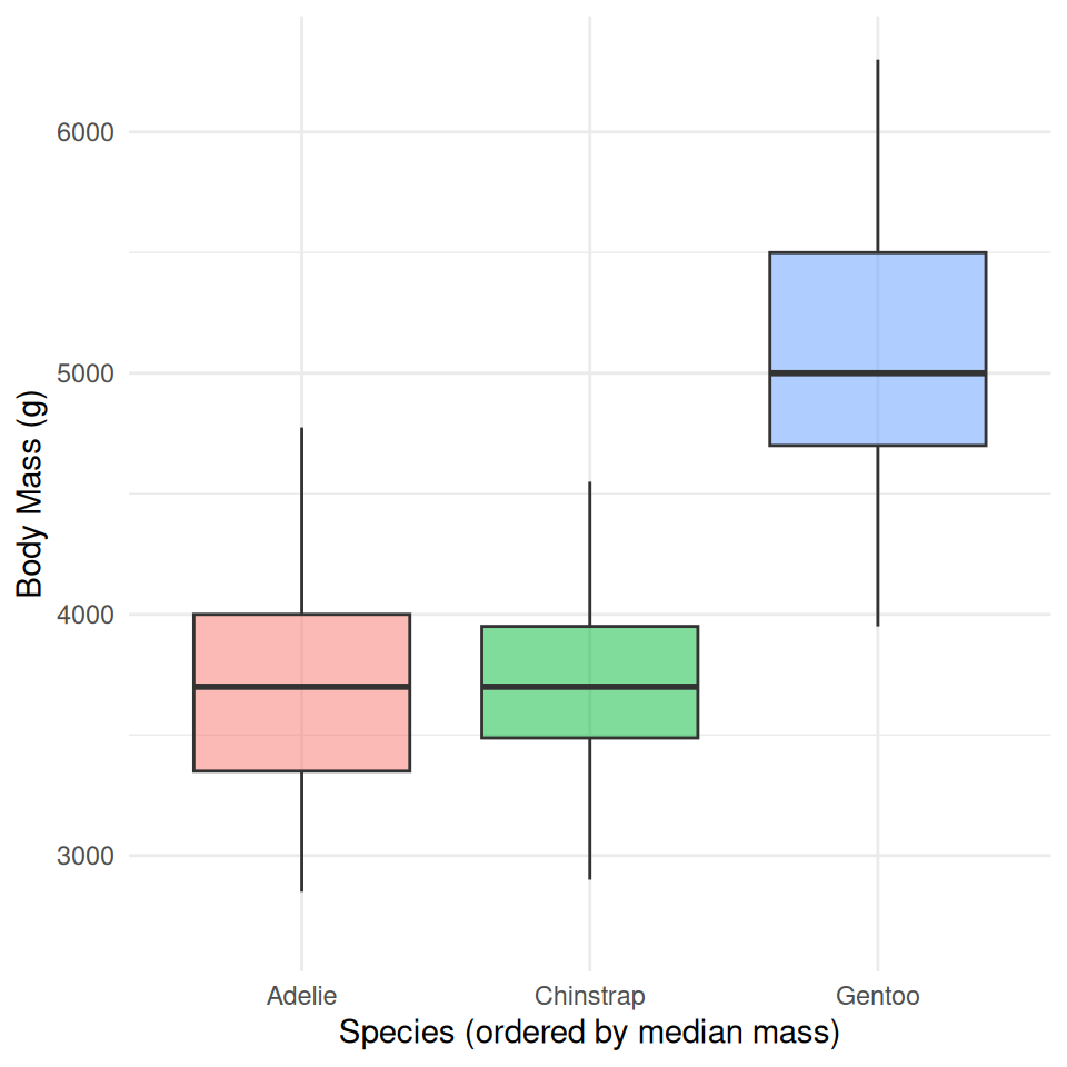

• fct_reorder(f, x, .fun = median) — reorder factor f by a summary of x
• Do it inside mutate(), then plot the result
• One line; the plot now reads lightest → heaviest

Tip

The full forcats family — rename levels, merge them, lump rare ones — is in Common Code 15 · Factors. Today we only need ordering and, next, the reference level.

🛑 Pause — Do Activity Parts 1–4 Now

Load the penguins, plot body mass by species, reorder the boxplot with fct_reorder(), and write your hypotheses. Predict which species differ before you run anything.

🧩 Chunk 2 of 2 · Fit the Model & Check Assumptions

We will cover: fitting the model, then checking normality of the residuals and equal variance across groups.

Tip

🖐 After this chunk: Activity Parts 5–8 (fit, set the reference level, QQ + Shapiro on residuals, Levene’s test).

Fit the Model

# ANOVA is a linear model with a categorical X ---------
mass_model <- lm(body_mass_g ~ species, data = penguins_df)

• lm(Y ~ X) — the same syntax as regression (Lecture 11)
• When X is categorical, that linear model is a one-way ANOVA
• We check assumptions on this model before reading any p-value

Note

✅ Key idea

lm(body_mass_g ~ species) is the exact same function call you used for a numeric predictor in Lecture 11 — only species is categorical this time. R handles the encoding automatically; you don’t write anything differently to get an ANOVA instead of a regression.

📖 W&S §15.2

Which Group Is the Baseline? — fct_relevel()

# The (Intercept) is the FIRST level = Adelie ---------
coef(mass_model)

     (Intercept) speciesChinstrap    speciesGentoo 
      3700.66225         32.42598       1375.35401 

# Make Gentoo the reference instead --------------------
penguins_relevel <- penguins_df %>%
  mutate(species = fct_relevel(species, "Gentoo"))

coef(lm(body_mass_g ~ species, data = penguins_relevel))

     (Intercept)    speciesAdelie speciesChinstrap 
        5076.016        -1375.354        -1342.928 

• lm picks the first factor level as the baseline; every coefficient is a difference from that group
• fct_relevel(species, "Gentoo") moves Gentoo to the front → coefficients are now differences from Gentoo

Important

Releveling changes which comparisons the coefficients show. It does not change the overall F or p-value — the ANOVA question (“do any means differ?”) is the same no matter which group you call the baseline.

Assumption 1 — Normality of the Residuals

Note

🔮 Predict first: plot(mass_model) gives the same four panels you saw in the regression lecture. With ~340 penguins instead of 118 near-perfect paper squares, do you expect the Normal Q-Q panel to track the line as tightly?

# Same plot(model) diagnostics as Lecture 11's regression
par(mfrow = c(2, 2))
plot(mass_model)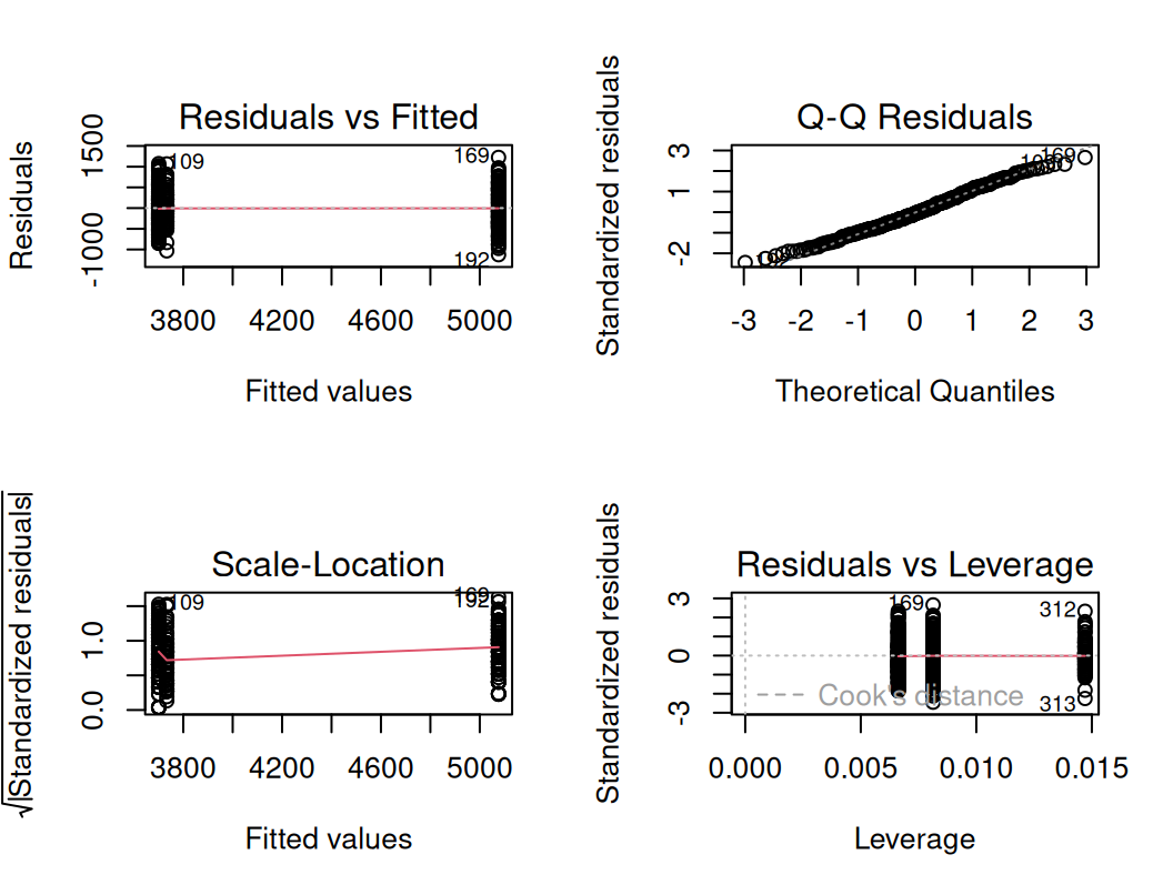

shapiro.test(residuals(mass_model))

    Shapiro-Wilk normality test

data:  residuals(mass_model)
W = 0.99166, p-value = 0.05118

• Check normality of the residuals, not the raw masses
• Panel 2 (Normal Q-Q) is the main visual tool; Shapiro-Wilk is a formal companion
• Panels 1 & 3 double-check equal variance — the same job Levene’s does next, from a different angle

Important

Large-sample caution: with ~340 birds, Shapiro-Wilk flags tiny departures as “significant.” Trust the Q-Q panel — if points track the line, you’re fine.

Assumption 2 — Equal Variance (Levene’s Test)

Note

🔮 Predict first: Look back at the boxplot spreads. Predict — will Levene’s test call the variances equal (p > 0.05) or unequal?

# Levene's test — H0: all groups have equal variance --
leveneTest(body_mass_g ~ species, data = penguins_df)

Levene's Test for Homogeneity of Variance (center = median)
       Df F value   Pr(>F)   
group   2  5.1203 0.006445 **
      339                    
---
Signif. codes:  0 '***' 0.001 '**' 0.01 '*' 0.05 '.' 0.1 ' ' 1

• p > 0.05 → variances similar → classic ANOVA is fine
• p < 0.05 → variances differ → use Welch’s ANOVA:

oneway.test(body_mass_g ~ species,
            data = penguins_df,
            var.equal = FALSE)

Same spirit as Welch’s t-test — robust when spreads differ.

🛑 Pause — Do Activity Parts 5–8 Now

Fit lm(body_mass_g ~ species), set the reference level with fct_relevel(), check the residual QQ plot + Shapiro, and run Levene’s test. Predict each result before you run it.

What We Learned Today

Concepts:

• Many t-tests inflate the false-positive rate — ANOVA asks once
• F = between-group ÷ within-group variance (signal ÷ noise)
• A factor’s level order sets the plot order and the model baseline
• ANOVA is a linear model with a categorical predictor — same lm() as regression
• Assumptions: normal residuals, equal variance (Levene)

R skills:

• fct_reorder() to order groups by the response; fct_relevel() to set the baseline
• lm(Y ~ group)
• plot(model) diagnostics, shapiro.test(residuals())
• leveneTest()
• rest of the fct_* family → Common Code 15 · Factors

References:

• 📖 W&S Ch. 15 — ANOVA
• 📖 R4DS Ch. 16 — Factors

Up next — Lecture 14:

• Assumptions are checked — now we run the test
• aov() and car::Anova(), then emmeans post-hoc to find which species differ, and how to report it